set.seed(31415) # Seed for replication
gx <- function(x) { exp(x^2) } # Function to estimate
m <- 10^7 # Points to draw

mean(gx(runif(m))) # Use the integral approximation
[1] 1.462964‘Integration by Darts’
Suppose that you, for one reason or another, need to compute \[\int_{0}^{1}e^{x^2}dx.\] You may recognize \(e^{x^2}\) as one of the lovely functions which does not have an explicit anti-derivative, which leaves us trapped analytically. There are plenty of numerical methods for solving integrals – some of which you may have seen before – but we want to take a statistically motivated version. If we recall that, for \(X \sim \text{Unif}(0,1)\), its density \(f(x) = 1\) on \([0,1]\), then rewriting \[\int_{0}^{1}e^{x^2}dx = \int_{0}^{1}e^{x^2}(1)dx = \int_{0}^{1}e^{x^2}f(x)dx = E[e^{X^2}],\] provides some potentially interesting insight into a manner of approximating this integral.
Notably, estimating the value of this integral can be seen as equivalent to estimating \(E[e^{X^2}]\), where \(X \sim \text{Unif}(0,1)\). Generally speaking, we know that, given a sample \(X_1,\dots,X_m\), a reasonable estimator for \(E[g(X)]\) is simply \[\frac{1}{m}\sum_{i=1}^m g(X_i),\] and so we can write that \[\int_{0}^{1}e^{x^2}f(x)dx \approx \frac{1}{m}\sum_{i=1}^m e^{U_i^2},\] where \(U_i\stackrel{iid}{\sim}\text{Unif}(0,1)\). We can appeal to the Strong Law of Large Numbers (SLLN) to make this approximation more concrete. We know that, supposing \(E[e^{X^2}] < \infty\), as \(m\to\infty\), \[P\left(\lim_{m\to\infty}\left|\frac{1}{m}\sum_{i=1}^m e^{X_i^2} - \int_{0}^{1}e^{x^2}dx\right| < \epsilon\right) = 1.\]
We can implement this technique very quickly in R code as well. The value of this integral is, in fact, approximately \(1.46265\).
set.seed(31415) # Seed for replication
gx <- function(x) { exp(x^2) } # Function to estimate
m <- 10^7 # Points to draw
mean(gx(runif(m))) # Use the integral approximation[1] 1.462964As a result, with this fairly simple idea, and small amount of R code, we can readily estimate an (otherwise intractable) integral expression. This technique, applied broadly, is known as Monte Carlo integration.
If \(f(x)\) is a density function, supported on some interval \([a,b]\), then we know that \[\int_{a}^b g(x)f(x)dx = E[g(X)].\] We also know, from the SLLN, that, as \(m\to\infty\) \[\frac{1}{m}\sum_{i=1}^m g(X_i) \stackrel{a.s.}{\longrightarrow} E[g(X)].\] Combined together, if we wish to solve any integral of the form \[\int_{a}^b g(x)f(x)dx,\] then we can approximate this to arbitrary precision by sampling \(X_i \stackrel{iid}{\sim} f\), and computing the empirical average over \(i=1,\dots,m\). As we take larger and larger samples, we can estimate more and more precisely the intended integral.
For instance, suppose that we wish to \[\int_{2}^{4}\frac{e^{-x}}{2}dx = E[e^{-X}],\] where \(X \sim \text{Unif}(2,4)\). We can solve this integral analytically by hand, noting that the anti-derivative of \(e^{-x}/2 = -e^{-x}/2\), and so this will ultimately equate to \(\dfrac{e^{-2}-e^{-4}}{2}\), which is approximately 0.0585. Using R, we can approximate this integral for increasing values of \(m\) as follows.
set.seed(31415)

ms <- c(10, 10^2, 10^3, 10^4, 10^5, 10^6, 10^7, 10^8)
fx <- function(x) { exp(-x) }

# Use the 'sapply' function to increase efficiency slightly
# We want to take the mean, of fx applied to runif for the correct number
estimated_vals <- sapply(ms, FUN = function(m) {
  mean(fx(runif(m, min = 2, max = 4)))
})

plot(x = ms,
     y = estimated_vals,
     log = "x",
     ylab = "Estimated Value",
     xlab = "Monte Carlo replicates (m; log scale)",
     main = "Monte Carlo Integration")
abline(h = (exp(-2)-exp(-4))/2, lty = 3)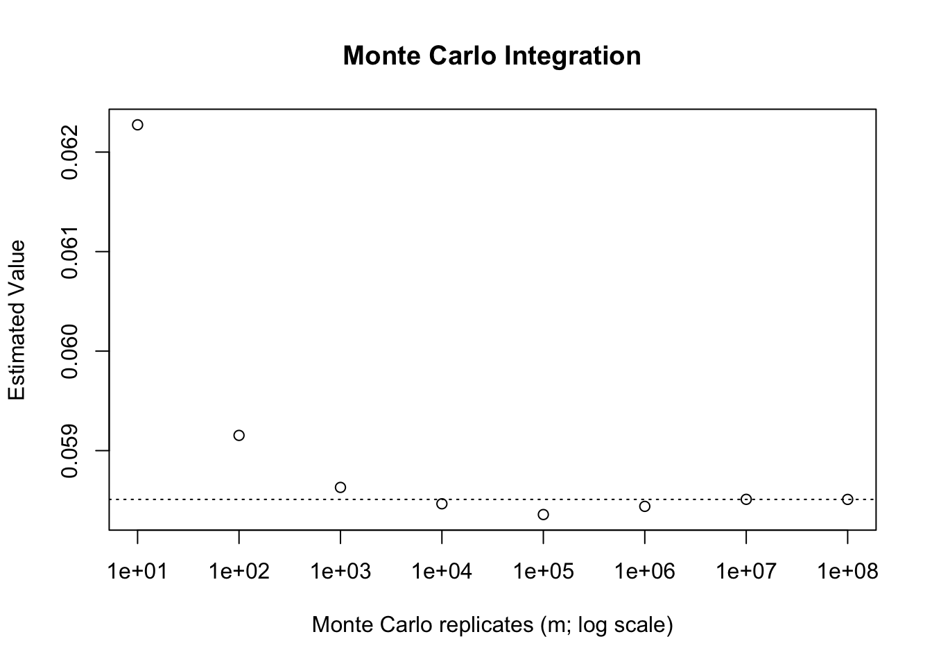
While the concept has been motivated whenever we wish to integrate the product of a function, \(g(x)\) by a density, \(f(x)\), over the full support of that random variable, most times we are presented with an integral we will not have it take the form of \(g(x)f(x)\). In these cases, we can use the only trick that statisticians have for performing integration: introduce a density. In particular, if we have any proper, definite integral (which is to say, any integral defined on an intervals \([a,b]\)) then we are always able to introduce the density for \(X \sim \text{Unif}(a,b)\). Specifically, \[f(x) = \frac{1}{b-a}, \quad x\in[a,b],\] and so we can write \[\int_{a}^{b} g(x)dx = (b-a)\int_{a}^{b}g(x)\frac{1}{b-a}dx = (b-a)E[g(X)].\]
Suppose, for instance, that we wish to integrate \(\dfrac{1}{1+x^2}\) from \(x = -2\) to \(3\). We can write \[\int_{-2}^{3} \frac{1}{1+x^2}dx = 5\int_{-2}^{3}\frac{1}{5(1+x^2)}dx = 5E\left[\frac{1}{1+X^2}\right],\] where \(X \sim \text{Unif}(-2, 3)\). This integral is given by \(\arctan(2) + \arctan(3)\), which is approximately 2.3562. Once again, we can implement a fairly simple Monte Carlo approximation to this.
set.seed(31415)

ms <- c(10, 10^2, 10^3, 10^4, 10^5, 10^6, 10^7, 10^8)
fx <- function(x) { 1/(1+x^2) }

# Compute the averages applied across the various values of 'm'
# Remember to multiply by 5!
estimated_vals <- sapply(ms, FUN = function(m) {
  5 * mean(fx(runif(m, min = -2, max = 3)))
})

plot(x = ms,
     y = estimated_vals,
     log = "x",
     ylab = "Estimated Value",
     xlab = "Monte Carlo replicates (m; log scale)",
     main = "Monte Carlo Integration")
abline(h = atan(2) + atan(3), lty = 3)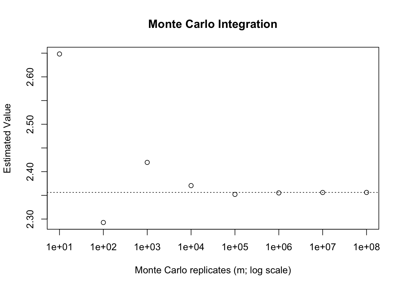
Sometimes we may have improper integrals (with limits at \(\pm\infty\) either one or both). In these cases we cannot use a uniformly distributed random variable to apply Monte Carlo techniques since the \(\text{Uniform}(a, \infty)\) is not well defined. There are times where Monte Carlo techniques may still be applicable, either by leveraging an infinitely supported random variable for the density, or else through integration tricks. Suppose, continuing from the previous example, that we wish to solve the improper integral \[\int_{0}^\infty \frac{1}{1+x^2}dx.\] If we wish to use a random variable supported on \([0,\infty)\) we may think to take \(X \sim \text{Exp}(1)\). The density of \(X\) is \(e^{-x}\). As a result, we can write \[\int_{0}^\infty \frac{1}{1+x^2}dx = \int_{0}^\infty \frac{1}{e^{-x}(1+x^2)}e^{-x}dx = E\left[\frac{e^x}{(1+x^2)}\right].\] Then, applying the procedure sampling from \(\text{Exp}(1)\) will allow us (in theory) to compute this integral.
set.seed(31415)

ms <- c(10, 10^2, 10^3, 10^4, 10^5, 10^6, 10^7, 10^8)
fx <- function(x) { exp(x)/(1+x^2) }

# Compute the averages applied across the various values of 'm'
estimated_vals <- sapply(ms, FUN = function(m) {
  mean(fx(rexp(m)))
})

plot(x = ms,
     y = estimated_vals,
     log = "x",
     ylab = "Estimated Value",
     xlab = "Monte Carlo replicates (m; log scale)",
     main = "Monte Carlo Integration")
abline(h = pi/2, lty = 3)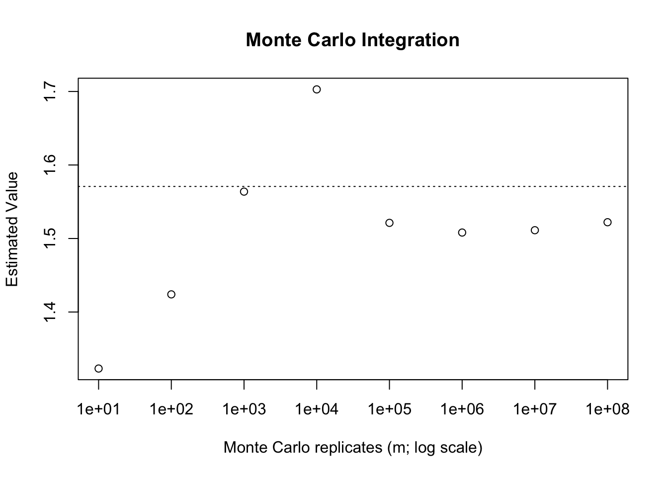
We can see that, compared to our previous attempts this is not a particularly effective approach. Even with \(m=10^8\) samples we still see sizable error versus the true value. We will understand why this is the case later on, however, the basic idea is that \(\text{Exp}(1)\) is not viable density to choose in this case.1 In fact, this density is theoretically invalid for this purpose. See if you can think of why, by considering the quantity that we are actually computing here.
As an alternative integral that we may wish to compute would be \(\Phi(x)\) which is given by \[\Phi(x) = P(Z\leq x) = \int_{-\infty}^x \frac{1}{\sqrt{2\pi}}e^{-t^2/2}dt.\] Here we can use symmetry properties of the normal distribution to note that \[\int_{-\infty}^0 \frac{1}{\sqrt{2\pi}}e^{-t^2/2}dt = 0.5,\] and thus \[\Phi(x) = 0.5 + \int_{0}^x \frac{1}{\sqrt{2\pi}}e^{-t^2/2}dt.\] Note that if \(x < 0\), \[\int_{0}^x \frac{1}{\sqrt{2\pi}}e^{-t^2/2}dt = -\int_{0}^{|x|} \frac{1}{\sqrt{2\pi}}e^{-t^2/2}dt,\] and so we can consider \(x > 0\) and simply subtract the resulting integral if \(x < 0\). To approximate this, we could use \(\text{Unif}(0,x)\) to compute this, multiplying through by \(x\). This may be undesirable if, for instance, we wanted to be able to prepare the generated random numbers in advance. We may think of using a change of variable, say \(y = \dfrac{t}{x}\), which makes the endpoints of integration \([0,1]\). Working through we get \(dy = \frac{1}{x}dt\), and so \[\Phi(x) = 0.5 + \int_{0}^x \frac{1}{\sqrt{2\pi}}e^{-t^2/2}dt = 0.5 + \int_{0}^1 \frac{x}{\sqrt{2\pi}}e^{-(xy)^2/2}dy = 0.5 + \frac{x}{\sqrt{2\pi}}\int_{0}^1e^{-(xy)^2/2}dy.\] This then allows us to use \(\text{Unif}(0,1)\).
We can consider doing this for various values of \(x\). The following table includes results for \(m=10^6\), comparing this Monte Carlo approximation to values computed using the pnrom function.
set.seed(31415)

m <- 10^6
xs <- seq(-3, 3, length.out = 10)
fxy <- function(x, y) { exp(-(x*y)^2/2) }

# Compute the averages applied across the various values of 'x'
estimated_vals <- sapply(xs, FUN = function(x) {
 u <- runif(m)
 0.5 + mean(fxy(x = x, y = u))*x/sqrt(2*pi)
})

# Output the Table
kableExtra::kable_styling(
  knitr::kable(
    data.frame("X" = xs,
               "Phi(X)" = round(pnorm(xs), 4),
               "MC-Phi(X)" = round(estimated_vals, 4), check.names = FALSE),
    align = c("c","c","c"),
    table.attr = 'data-quarto-disable-processing="true"'
  ),
  bootstrap_options = c("striped"), full_width = FALSE
)| X | Phi(X) | MC-Phi(X) |
|---|---|---|
| -3.0000000 | 0.0013 | 0.0023 |
| -2.3333333 | 0.0098 | 0.0096 |
| -1.6666667 | 0.0478 | 0.0478 |
| -1.0000000 | 0.1587 | 0.1587 |
| -0.3333333 | 0.3694 | 0.3694 |
| 0.3333333 | 0.6306 | 0.6306 |
| 1.0000000 | 0.8413 | 0.8414 |
| 1.6666667 | 0.9522 | 0.9519 |
| 2.3333333 | 0.9902 | 0.9898 |
| 3.0000000 | 0.9987 | 0.9986 |
We can see from the results here that the Monte Carlo technique matches the numerical integration well for most of the values of \(x\) within the main part of the density. For the tail values we see a larger discrepancy, though, the approximation still seems to work mostly well.
In the previous example we wanted to integrate \(\Phi(x)\). An alternative approach to this is known as the hit-or-miss technique. Suppose that \(I(\cdot)\) is the indicator function (i.e., it takes a value of \(1\) if its argument holds, and \(0\) otherwise). We can view \(\Phi(x) = E[I(Z \leq x)]\), since \[E[I(Z \leq x)] = \int_{-\infty}^\infty I(z \leq x)\frac{1}{\sqrt{2\pi}}e^{-t^2/2}dt = \int_{-\infty}^x (1)\frac{1}{\sqrt{2\pi}}e^{-t^2/2}dt + \int_{x}^\infty = \Phi(x).\] We know that \[\frac{1}{m}\sum_{i=1}^m I(Z \leq x) \stackrel{a.s.}{\longrightarrow} E[I(Z \leq x)] = \Phi(x),\] and so this gives another approach to this integral. Specifically, we can generate \(Z_i \sim N(0,1)\) and then simply compute the average of the desired indicator function. This is the same as the proportion below the threshold, and is incidentally, using the empirical CDF to estimate the true CDF.
m <- 10^6
xs <- seq(-3, 3, length.out = 10)
fxy <- function(x, y) { y <= x }

# Compute the averages applied across the various values of 'x'
estimated_vals_hitmiss <- sapply(xs, FUN = function(x) {
 Z <- rnorm(m)
 mean(fxy(x = x, y = Z))
})

# Output the Table
kableExtra::kable_styling(
  knitr::kable(
    data.frame("X" = xs,
               "Phi(X)" = round(pnorm(xs), 4),
               "MC-Phi(X)" = round(estimated_vals, 4),
               "MC-Phi-HM(X)" = round(estimated_vals_hitmiss, 4),
               check.names = FALSE),
    align = c("c","c","c"),
    table.attr = 'data-quarto-disable-processing="true"'
  ),
  bootstrap_options = c("striped"), full_width = FALSE
)| X | Phi(X) | MC-Phi(X) | MC-Phi-HM(X) |
|---|---|---|---|
| -3.0000000 | 0.0013 | 0.0023 | 0.0013 |
| -2.3333333 | 0.0098 | 0.0096 | 0.0098 |
| -1.6666667 | 0.0478 | 0.0478 | 0.0478 |
| -1.0000000 | 0.1587 | 0.1587 | 0.1590 |
| -0.3333333 | 0.3694 | 0.3694 | 0.3688 |
| 0.3333333 | 0.6306 | 0.6306 | 0.6306 |
| 1.0000000 | 0.8413 | 0.8414 | 0.8412 |
| 1.6666667 | 0.9522 | 0.9519 | 0.9522 |
| 2.3333333 | 0.9902 | 0.9898 | 0.9901 |
| 3.0000000 | 0.9987 | 0.9986 | 0.9986 |
This approach seems to mirror a type of acceptance-rejection sampling, of sorts. In fact, this technique itself can be used to estimate the area of any boundable shape. Suppose that we have a shape which can be inscribed into a rectangular area, \([a,b]\times[c,d]\). If we want to know the area of this shape one technique would be to use the hit-or-miss technique. We could generate \(x = \text{Unif}(a,b)\) and \(y = \text{Unif}(c,d)\). Then, if we take \(g(x, y) = I((x,y)\in A)\), where \(A\) defines the shape of interest, we can approximate \(P((X,Y) \in A) = E[I((X,Y)\in A)]\) via Monte Carlo techniques. We know that theoretically, \[P((X,Y) \in A) = \frac{\text{Area}(A)}{(b-a)\times (d-c)},\] and so multiplying the estimated proportion of points that fall within the shape by the area of the bounding rectangle, we can estimate the particular area of interest.
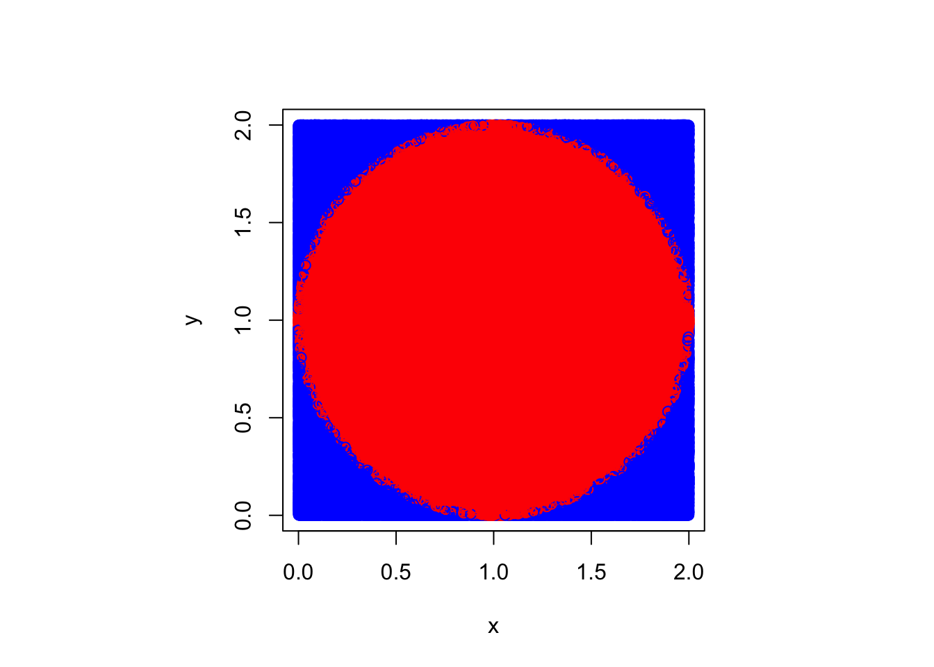
A common demonstration of this technique is to use Monte Carlo techniques to estimate the value of \(\pi\). Suppose we inscribe a circle into the square on \([0,2]\times[0,2]\), which is to say the circle is centered at \((1,1)\) and has radius \(1\). We know that the area of this circle is \(\pi r^2 = \pi\). The area of the square is \(4\), and so \(4\) times the estimated proportion that fall into this will approximate \(\pi\). Note that any point \((x,y)\) in the circle will satisfy \(\sqrt{(x-1)^1 + (y-1)^2} \leq 1\), and so we can use this as the indicator expression. Taken together, we have the following technique for estimating the value of \(\pi\).
set.seed(31415)

m <- 10^6

# Generate Random Points
x <- runif(m, 0, 2)
y <- runif(m, 0, 2)

# Estimate Pi as the Proportion in the Circle times 4
4 * mean((x - 1)^2 + (y - 1)^2 <= 1)
[1] 3.142548Graphically, we can think of colouring the “hits” in, in red, and leaving the misses in blue.
Because the numerical approximation relies on random number generation, we can view each of our Monte Carlo integrals as an estimator. These estimators are all unbiased, by construction, and as a result assessing them is equivalent to assessing their variance. All else equal, we prefer an estimator with a lower variance. In the case of using \[\frac{1}{m}\sum_{i=1}^n g(X_i)\] as our estimator, we find that the variance is given by \[\text{var}\left(\frac{1}{m}\sum_{i=1}^n g(X_i)\right) = \frac{1}{m^2}\sum_{i=1}^m \text{var}(g(X_i)) = \frac{1}{m}\text{var}(g(X_i)),\] so long as the \(X_i\) are all independent and identically distributed. Depending on \(g(X_i)\), we may be able to directly solve for this value, and if not, we can estimate it using \[\frac{1}{m}\sum_{i=1}^m (g(X_i) - \overline{g(X_i)})^2.\] This is simply the sample variance of the function \(g(X)\).2
In addition to being able to directly estimate the variance or standard error, we can also use this same process to apply techniques from inference. Notably, if \(m\) is large enough, and our estimator has finite variance, then (using \(\widehat{\theta}\) as the Monte Carlo estimator of \(\theta\)), \[\frac{\widehat{\theta} - \theta}{\sqrt{\text{var}(\widehat{\theta})}} \stackrel{d}{\longrightarrow} N(0,1).\] This allows for approximate confidence intervals to be formed, which give us a technique for producing error estimates or quantifying our uncertainty directly.
For instance, suppose that we consider the hit-or-miss technique for estimating \(\Phi(x)\). We know that \(g(Z) = I(Z \leq x)\) is going to be a Bernoulli random variable, and so the variance is given by \(P(Z\leq x)(1 - P(Z \leq x)) = \Phi(x)(1 - \Phi(x))\). We do not know \(\Phi(x)\) and so instead we can choose to use the conservative estimate of \(\Phi(x) = 0.5\); that is, \(\text{var}(g(Z)) \leq 0.25\). Taken together then, \(\text{var}(\widehat{\theta}) \leq \dfrac{1}{4m}\), and so we can use this to estimate say a \(99\%\) confidence interval around the truth.
m <- 10^6

# Output the Table
kableExtra::kable_styling(
  knitr::kable(
    data.frame("X" = xs,
               "Phi(X)" = round(pnorm(xs), 4),
               "MC-Phi(X)" = round(estimated_vals, 4),
               "MC-Phi-HM-LB" = round(estimated_vals_hitmiss - qnorm(0.995) / (2*sqrt(m)), 4),
               "MC-Phi-HM(X)" = round(estimated_vals_hitmiss, 4),
               "MC-Phi-HM-UB" = round(estimated_vals_hitmiss + qnorm(0.995) / (2*sqrt(m)), 4),
               check.names = FALSE),
    align = c("c","c","c"),
    table.attr = 'data-quarto-disable-processing="true"'
  ),
  bootstrap_options = c("striped"), full_width = FALSE
)| X | Phi(X) | MC-Phi(X) | MC-Phi-HM-LB | MC-Phi-HM(X) | MC-Phi-HM-UB |
|---|---|---|---|---|---|
| -3.0000000 | 0.0013 | 0.0023 | 0.0001 | 0.0013 | 0.0026 |
| -2.3333333 | 0.0098 | 0.0096 | 0.0085 | 0.0098 | 0.0111 |
| -1.6666667 | 0.0478 | 0.0478 | 0.0465 | 0.0478 | 0.0491 |
| -1.0000000 | 0.1587 | 0.1587 | 0.1578 | 0.1590 | 0.1603 |
| -0.3333333 | 0.3694 | 0.3694 | 0.3675 | 0.3688 | 0.3701 |
| 0.3333333 | 0.6306 | 0.6306 | 0.6294 | 0.6306 | 0.6319 |
| 1.0000000 | 0.8413 | 0.8414 | 0.8399 | 0.8412 | 0.8425 |
| 1.6666667 | 0.9522 | 0.9519 | 0.9509 | 0.9522 | 0.9534 |
| 2.3333333 | 0.9902 | 0.9898 | 0.9888 | 0.9901 | 0.9914 |
| 3.0000000 | 0.9987 | 0.9986 | 0.9973 | 0.9986 | 0.9999 |
All else equal, we would like the lowest variance Monte Carlo estimator. As a result, it is worth considering various techniques which may allow us to achieve this goal. First, suppose that we have two estimators, \(\widehat{\theta}_1\) and an improved \(\widehat{\theta}_2\). We will either think about the relative effiency of these two estimators, or else the percent reduction in variance moving to estimator \(\widehat{\theta}_2\). For relative efficiency we take \[\text{R.E}(\widehat{\theta}_1, \widehat{\theta}_2) = \frac{\widehat{\theta}_1}{\widehat{\theta}_2},\] and if \(\text{R.E} < 1\) then \(\widehat{\theta}_1\) is preferred (and vice versa). To get the percent reduction in variance, we can take \[100\left(\frac{\text{var}(\widehat{\theta}_1) - \text{var}(\widehat{\theta}_2)}{\text{var}(\widehat{\theta}_1)}\right).\]
One technique to lower the variance of an estimator is to simply increase \(m\). If we think about computing \(\widehat{\theta}_1\) using \(m\) replicates and then \(\widehat{\theta}_2\) with the same process and \(cm\) replicates, the relative efficiency, \(\text{R.E.}(\widehat{\theta}_1, \widehat{\theta}_2) = c\), and the percent reduction in variance is \(\dfrac{100(c-1)}{c}\). As a result, if you want to reduce the standard error by an order of magnitude, you will need to take \(c=100\). For two orders of magnitude, you would need \(c=10000\). This becomes quite untenable, quite quickly, as a reliable technique for reducing the overall variance. As a result, we would like to consider alternative techniques wherever possible. What follows are several such techniques.
For two arbitrary random variables, \(U_1\) and \(U_2\) we know that the variance \(\text{var}(U_1 + U_2) = \text{var}(U_1) + \text{var}(U_2) + 2\text{cov}(U_1, U_2)\). Whenever we assume that \(U_1 \perp U_2\) then the covariance term is \(0\) and we have just the summation of the two individual variances. If we knew that \(\text{cov}(U_1, U_2) < 0\) then the variance of \(U_1 + U_2\) would be less than the variance of two independent variables being summed, with otherwise equal variances. In the case of our Monte Carlo estimation, if there was a way to make the \(g(X_i)\) negatively correlated then this would permit an overall variance reduction. One technique for doing this is to use so-called antithetic variables.
If \(U_1 \sim \text{Unif}(0,1)\), then \(1 - U_1 \sim \text{Unif}(0,1)\) as well. To see this note that \[P(1 - U_1 \leq k) = P(1 - k \leq U_1) = 1 - P(U_1 \leq 1-k) = 1- (1-k) = k.\] Thus, if we generate \(U_1 \sim \text{Unif}(0,1)\), then \(1 - U_1\) is also uniform. However, consider the covariance between these two random variables. \[\text{cov}(U_1, 1 - U_1) = -\text{cov}(U_1, U_1) = -\text{var}(U_1).\] As a result, they are negatively correlated. In fact, \(U_1 + (1 - U_1)\) will always have variance \(0\). Suppose that we are then computing \(Y_1 = g(U_1)\) and \(Y_2 = g(1 - U_1)\) as two terms in the Monte Carlo summation. One can show3 that if \(g\) is monotone (either increasing or decreasing), \(Y_1\) and \(Y_2\) will be negatively correlated. This gives us an alternative approach to performing Monte Carlo integration with a reduced variance. First, we generate \(m/2\) random variables from a \(\text{Unif}(0,1)\) distribution. Then we fill out the sample using \(1-u_i\) for each \(i=1,\dots,m/2\). Then, as long as \(g\) is monotone, computing \[\widehat{\theta} = \frac{1}{m}\sum_{i=1}^{m/2}\left(g(u_i) + g(1 - u_i)\right)\] will have a variance reduced relative to the standard estimator.
It is worth considering what happens if, as is often the case, our Monte Carlo techniques require \(X_i\) not from a \(\text{Unif}(0,1)\) distribution. In this case, we can still apply antithetic variables if \(X_i = F^{-1}(U_i)\) (which is to say, it is generated through the inverse transformation technique). We know that \(F^{-1}\) is a monotonic function, and as a result, \(F^{-1}(U)\) and \(F^{-1}(1 - U)\) will be negatively correlated, and then we can apply the same argument as above to \(X_i\) in place of \(U_i\).
We have been considering the estimation of \(\Phi(x)\). Prior to the hit-or-miss technique, we saw a version of the estimator that relied on \(U(0,1)\) sampling, by using Monte Carlo estimation on the residual portion of the integral (after using symmetry tricks). In particular, we consider \(\int_{0}^1 e^{-(xy)^2/2}dy\). Note that on \([0,1]\) \(e^{-(xy)^2/2}\) is monotonic, and so we should expect a reduction in the variance. We consider repeating Monte Carlo estimation of this \(200\) times to get a sense of the variability of the estimators.
repeat_experiment <- 200

set.seed(31415)

m <- 10^5
half_m <- m / 2
fxy <- function(x, y) { exp(-(x*y)^2/2) }

results <- matrix(0,
                  nrow = repeat_experiment,
                  ncol = 2)

# Repeat the Experiment Many Times to Get a Sense of Variability
for(ii in 1:repeat_experiment) {
  # Standard version
  standard <- mean(fxy(x = 1.5, y = runif(m)))

  # Antithetic Version
  U <- runif(half_m)
  antithetic <- mean(fxy(x = 1.5, y = c(U, 1 - U)))

  results[ii, ] <- c(standard, antithetic)
}

colnames(results) <- c("Standard MC", "Antithetic MC")

boxplot(results, main = "Standard and Antithetic MC Integration")
abline(h = (pnorm(1.5) - 0.5) * sqrt(2*pi) / 1.5, lty = 2)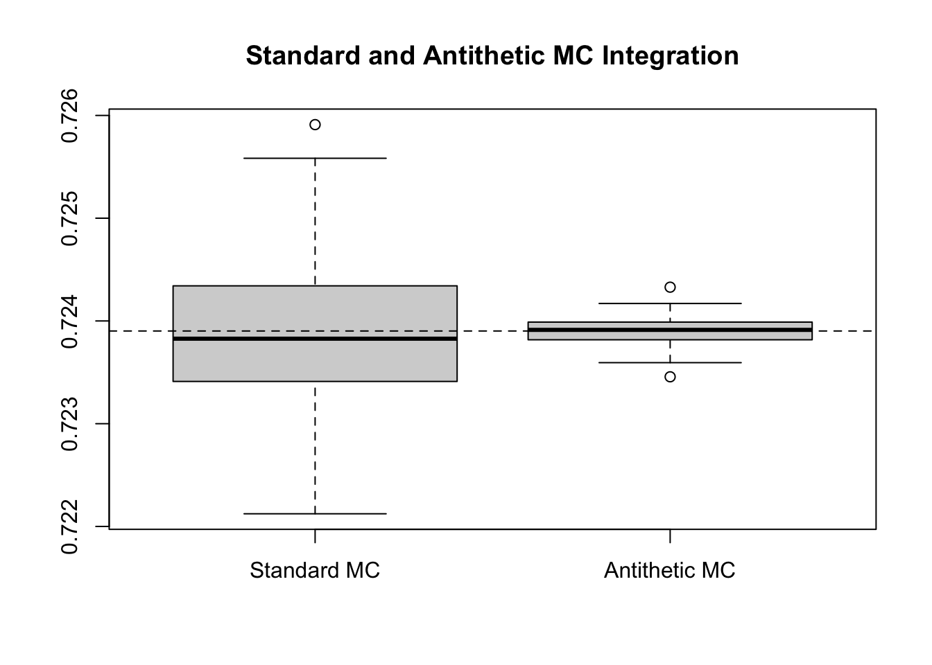
While the differences are visually apparent, we can compute the (estimated) relative efficiency and percent variance reduction as well. The estimated variance of the standard estimators is 0 compared to 0 for the antithetic. This corresponds to a relative efficiency of 32.2812 and a percent reduction of 96.9022%. To get a similar reduction based on increasing \(m\), we would have needed to use 3228122 samples, rather than the 100000 that were used. In fact, we can see this example in action.
repeat_experiment <- 200

set.seed(31415)

m1 <- 10^5
half_m1 <- m1 / 2
m2 <- 3228122
half_m2 <- m2 / 2
fxy <- function(x, y) { exp(-(x*y)^2/2) }

results <- matrix(0,
                  nrow = repeat_experiment,
                  ncol = 4)

# Repeat the Experiment Many Times to Get a Sense of Variability
for(ii in 1:repeat_experiment) {
  # Standard version
  standard <- mean(fxy(x = 1.5, y = runif(m1)))

  # Antithetic Version
  U <- runif(half_m1)
  antithetic <- mean(fxy(x = 1.5, y = c(U, 1 - U)))

  # Standard version
  standard2 <- mean(fxy(x = 1.5, y = runif(m2)))

  # Antithetic Version
  U2 <- runif(half_m2)
  antithetic2 <- mean(fxy(x = 1.5, y = c(U2, 1 - U2)))

  results[ii, ] <- c(standard, antithetic, standard2, antithetic2)
}

colnames(results) <- c("Standard MC \n (Small m)",
                       "Antithetic MC \n (Small m)",
                       "Standard MC \n (Large m)",
                       "Antithetic MC \n (Large m)")

boxplot(results, main = "Standard and Antithetic MC Integration")
abline(h = (pnorm(1.5) - 0.5) * sqrt(2*pi) / 1.5, lty = 2)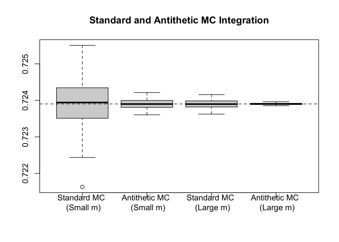
To see the importance of a monotonic \(g\), consider that earlier, saw the example of \[\int_{-2}^3 \frac{1}{1 + x^2}dx,\] using \(\text{Unif}(-2,3)\) random variables. We could have just as well transformed this, using the substitution \(t = \frac{x + 2}{5}\), to set the limits of integration to be \([0,1]\) and giving \(5dt = dx\). Then, \[\int_{-2}^3 \frac{1}{1 + x^2}dx = \int_{0}^1 \frac{1}{1 + (5t - 2)^2}5dt = E\left[\frac{5}{1 + (5U - 2)^2}\right],\] where \(U \sim \text{Unif}(0,1)\). Note that here, \(g\) is non-monotonic, and as a result, we will not expect variance reduction from the antithetic technique.
repeat_experiment <- 200

set.seed(31415)

m <- 10^5
half_m <- m / 2
fx <- function(x) { 5/(1+(5*x - 2)^2) }

results <- matrix(0,
                  nrow = repeat_experiment,
                  ncol = 2)

# Repeat the Experiment Many Times to Get a Sense of Variability
for(ii in 1:repeat_experiment) {
  # Standard version
  standard <- mean(fx(runif(m)))

  # Antithetic Version
  U <- runif(half_m)
  antithetic <- mean(fx(c(U, 1 - U)))

  results[ii, ] <- c(standard, antithetic)

}

colnames(results) <- c("Standard MC", "Antithetic MC")

boxplot(results, main = "Standard and Antithetic MC Integration")
abline(h = atan(2) + atan(3), lty = 3)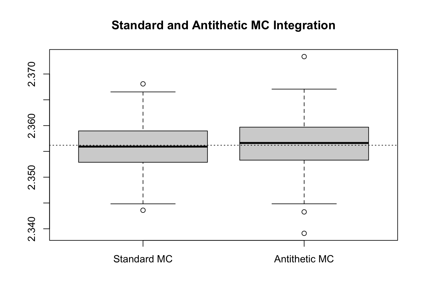
We can recast the process of using antithetic variables in a slightly different manner. Consider, instead of using \(m/2\) samples of \(u_i\) and the \(m/2\) samples of \(1-u_i\), that we compute \[\widehat{\theta}_1 = \frac{1}{m}\sum_{i=1}^m g(u_i).\] Then, in addition we compute \[\widehat{\theta}_2 = \frac{1}{m}\sum_{i=1}^m g(1 - u_i).\] Finally, we combine these two estimators using \[\widehat{\theta}_c = \widehat{\theta}_1 + c(\widehat{\theta}_2 - \widehat{\theta}_1) = c\widehat{\theta}_1 + (1-c)\widehat{\theta}_2.\] Note that \(\widehat{\theta}_c\) remains unbiased for \(\theta\), but that the total variance of this estimator is going to be \[c^2\text{var}(\widehat{\theta}_1) + (1-c)^2\text{var}(\widehat{\theta}_2) + c(1-c)\text{cov}(\widehat{\theta}_1,\widehat{\theta}_2).\] We know that \(\widehat{\theta}_1 \sim \widehat{\theta}_2\), by construction. If we consider that \(\text{cov}(\widehat{\theta}_1, \widehat{\theta}_2) = k\text{var}(\widehat{\theta}_1)\), for some \(|k| < 1\), then we get \[\text{var}(\widehat{\theta}_c) = (c^2 + (1-c)^2 + kc(1-c))\text{var}(\widehat{\theta}_1).\] If we want to figure out which value is optimal for \(c\) then we can take \(\dfrac{\partial}{\partial c}\) and solve this equal to zero, giving \[\frac{\partial}{\partial c} c^2 + (1-c)^2 + kc(1-c)) = 2c - 2(1-c) + k(1-2c) = 4c - 2ck + k - 2.\] This takes on an optimal value when \[4c - 2ck + k - 2 = 0 \iff 2c(2 - k) = 2 - k \iff c = \frac{1}{2}.\] Thus, the optimal value for \(c\) is \(\dfrac{1}{2}\), which gives exactly the estimators we had specified for the antithetic variables.
This formulation, however, hints at a subtle idea: if we take an estimator, say \(\widehat{\theta}_1\), we may be able to improve this estimator by adding to it another estimator which is correlated (and thus can reduce the variance). Notice that in the case of the above derivative we added \(c(\widehat{\theta}_2 - \widehat{\theta}_1)\). In general, if we add any quantity \(\Omega\) giving \(\widehat{\theta}_1 + \Omega\), then if this is to remain unbiased we must have \(E[\widehat{\theta}_1 + \Omega] = E[\widehat{\theta}_1] + E[\Omega] = E[\widehat{\theta}_1]\), and as a result \(\Omega\) requires expectation \(0\). This is true of \(c(\widehat{\theta}_2 - \widehat{\theta}_1)\) as \(E[\widehat{\theta}_2] = E[\widehat{\theta}_1]\). However, we can make this more general. Suppose that we have \(\widehat{\theta}_1 = g(X)\), then we can take \[\widehat{\theta}_c = g(X) + c(f(X) - E[f(X)]).\]
We can work out that, in this case, \[\text{var}(\widehat{\theta}_c) = \text{var}(g(X)) + c^2\text{var}(f(X)) + 2c\text{cov}(g(X), f(X)).\] If we wish to find the \(c\) that minimizes this variance, working through the same calculus steps gives \[\frac{\partial}{\partial c}\text{var}(g(X)) + c^2\text{var}(f(X)) + 2c\text{cov}(g(X), f(X)) = 2c\text{var}(f(X)) + 2\text{cov}(g(X), f(X)),\] which setting to \(0\) and solving gives \[c = -\frac{\text{cov}(g(X), f(X))}{\text{var}(f(X))}.\] At this value for \(c\), we find that the variance of \(\widehat{\theta}_c\) will be \[\text{var}(g(X)) - \frac{(\text{cov}(g(X), f(X)))^2}{\text{var}(f(X))},\] and so as long as \(g(X)\) and \(f(X)\) are correlated (positively or negatively) this will result in a reduced variance.
We refer to \(f(X)\) as a control variate and selecting a good control variate can result in a major variance reduction. Note that one challenge in the application of this technique is that we need to be able to analytically compute \(E[f(X)]\) to apply the technique as proposed. There are ways around this (as we saw when framing the antithetic variables as control variates), however, as a general rule we want to select control variates which:
For instance, suppose we wish to evaluate \[\int_{0}^1 \log(1+x)dx\] using Monte Carlo techniques with draws from \(\text{Unif}(0,1)\). This integral can be readily computed by hand to be \(\log(4) - 1\), and so we need not apply Monte Carlo techniques. However, it is informative to see an application of control variates where we know the outcome. Here we have \(g(X) = \log(X)\), and a natural choice for \(f(X) = X\) since \(\text{var}(X) = \frac{1}{12}\), and \[\text{cov}(\log(1+X), X) = \int_{0}^1 \log(1+x)xdx - \int_{0}^1\log(1+x)dx\int_{0}^1xdx = \frac{3 - 2\log(4)}{4}.\] Correspondingly, the optimal value for \(c\) is \[c = -\frac{12(3 - 2\log(4))}{4} = -3(3 - 2\log(4)).\]
Implementing this we can compare the variance reduction which is possible here.
repeat_experiment <- 200

set.seed(31415)

m <- 10^3
gx <- function(x) { log(1 + x) }
fx <- function(x) { x }
Ef <- 1/2
const <- -3 * (3 - 2*log(4))


results <- matrix(0,
                  nrow = repeat_experiment,
                  ncol = 2)

# Repeat the Experiment Many Times to Get a Sense of Variability
for(ii in 1:repeat_experiment) {
  U <- runif(m)

  # Standard version
  standard <- mean(gx(U))

  # Control Variate Version
  control_v <- mean(gx(U) + const * (fx(U) - Ef))

  results[ii, ] <- c(standard, control_v)

}

colnames(results) <- c("Standard MC", "Control Variate MC")

boxplot(results, main = "Standard and Control Variate MC Integration")
abline(h = log(4) - 1, lty = 3)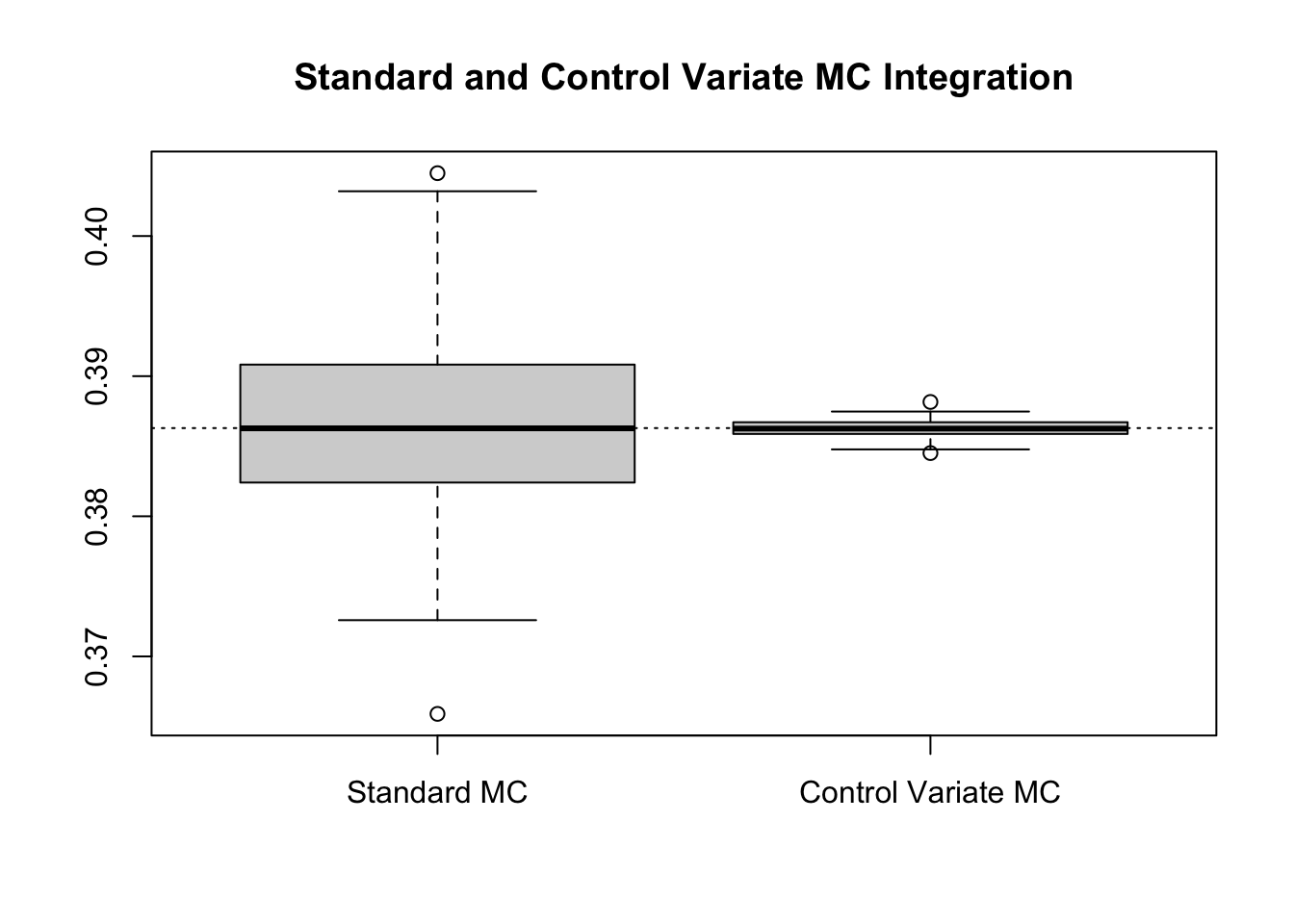
Numerically, this suggests a relative efficiency of 114.5532 and a percent reduction 99.127%.
While this is evidently a major reduction, this procedure has a major concern. Notably, the constant \(c\) depends on the covariance between \(g(X)\) and \(f(X)\). We are ultimately using this procedure to estimate \(E[g(X)]\) and so it will (generally) be quite unreasonable to assume that the covariance is available when the expected value is not. However, this can be overcome through the use of an estimated, based on a pilot Monte Carlo procedure. That is, we can generate one sample of \(X\), say \(X_1,\dots,X_{m'}\) and then use this sample to compute \(\text{cov}(g(X), f(X))\). Then, with this estimated value, we can compute the Monte Carlo procedure itself. Often we may be able to get away with a smaller value for \(m'\), and so if the computational cost of generating the extra variables is not too great, then this procedure can work well. If this is costly, it is also possible to estimate the covariance via the same runs that are used for the Monte Carlo techniques themselves. While this reducing the computational burden somewhat, it has the drawback of removing the unbiasedness of \(g(X) + \widehat{c}(f(X) - \mu)\), since now \(\widehat{c}\) depends on the same random variable, \(X\). This bias will go to zero as \(m\to\infty\). We will focus on the first, pilot data technique, but the alternative is worth exploring for certain situations.
Suppose in the previous example we did not know how to compute the covariance between \(\log(1+U)\) and \(U\), then we can use the following Monte Carlo approach. Note that if you did not know how to estimate \(\text{var}(f(X))\) either, the same pilot data can be used for that purpose.
repeat_experiment <- 200

set.seed(31415)

m <- 10^3
mp <- 10^5
gx <- function(x) { log(1 + x) }
fx <- function(x) { x }
Ef <- 1/2

# Pilot Work to Estimate 'c'
pilot_sample <- runif(mp)
cov_gf <- cov(gx(pilot_sample), fx(pilot_sample))
const <- -12 * cov_gf

results <- matrix(0,
                  nrow = repeat_experiment,
                  ncol = 2)

# Repeat the Experiment Many Times to Get a Sense of Variability
for(ii in 1:repeat_experiment) {
  U <- runif(m)

  # Standard version
  standard <- mean(gx(U))

  # Control Variate Version
  control_v <- mean(gx(U) + const * (fx(U) - Ef))

  results[ii, ] <- c(standard, control_v)

}

colnames(results) <- c("Standard MC", "Control Variate MC")

boxplot(results, main = "Standard and Control Variate MC Integration")
abline(h = log(4) - 1, lty = 3)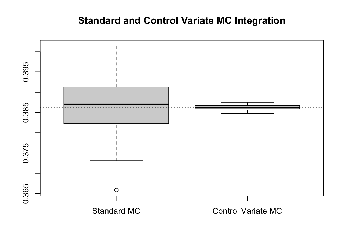
Numerically, this suggests a relative efficiency of 147.5161 and a percent reduction 99.3221%, results which match (or exceed) that of the known constant.
If you are brushed up on your linear regression knowledge, you may remember that the slope of a simple linear regression is given by \[\frac{\text{cov}(X,Y)}{\text{var}(X)}.\] That is, the optimal constant is simply the negative value of the slope of a linear regression of \(g(X) \sim f(X)\). To see this, consider the pilot sample we had previously. In this sample we can run a linear regression, and compare the result to -0.6840747.
linear_model <- lm(gx(pilot_sample) ~ fx(pilot_sample))
slope_coef <- coef(linear_model)["fx(pilot_sample)"]

-slope_coef
fx(pilot_sample)
-0.6819923 The slight discrepancy occurs because we did not estimate the variance in computing \(\widehat{c}\) previously. Had we, we would have gotten -0.6819923. What about the intercept? In a simple linear regression model, \[\widehat{\beta}_0 = \overline{y} + \widehat{\beta}_1\overline{x},\] and so converting to our setup we get \[\widehat{\beta}_0 = \overline{g(X)} - (-\widehat{c})\overline{f(X)}.\] The prediction equation for our linear regression model is thus \[\overline{g(X)} - (-\widehat{c})\overline{f(X)} + (-\widehat{c})x = \overline{g(X)} + \widehat{c}(\overline{f(X)} - x).\] Thus, if we predict the value for \(g(X)\) when \(f(X) = E[X]\), the prediction equation exactly equals the Monte Carlo equation for our control variate corrected value. To see this in action, consider the following.
set.seed(31415)

m <- 10^3
gx <- function(x) { log(1 + x) }
fx <- function(x) { x }

# Generate Uniform Sample
U <- runif(m)

# Fit Linear Regression Model
y <- gx(U)
x <- fx(U)
lr <- lm(y ~ x)
const <- -coef(lr)['x']

# Control Variate Version
control_v <- mean(gx(U) + const * (fx(U) - Ef))

# Linear Regression Predicted Version
lr_v <- predict(lr, newdata = data.frame(x = Ef))

c(control_v, unname(lr_v))
[1] 0.3864248 0.3864248If we want to know the estimated variance of the controlled random variate, or in fact the estimated reduction in variance from the control, we can get these via a call to the summary(...) method. The output from the summary is printed below.
summary(lr)
Call:
lm(formula = y ~ x)

Residuals:
      Min        1Q    Median        3Q       Max
-0.046403 -0.013330  0.004995  0.015872  0.019237

Coefficients:
            Estimate Std. Error t value Pr(>|t|)
(Intercept) 0.046428   0.001117   41.57   <2e-16 ***
x           0.679993   0.001938  350.94   <2e-16 ***
---
Signif. codes:  0 '***' 0.001 '**' 0.01 '*' 0.05 '.' 0.1 ' ' 1

Residual standard error: 0.01767 on 998 degrees of freedom
Multiple R-squared:  0.992, Adjusted R-squared:  0.992
F-statistic: 1.232e+05 on 1 and 998 DF,  p-value: < 2.2e-16
We can access the summary(...)$sigma^2 to estimate the variance of the Monte Carlo estimate (the $sigma property in turn gives the estimated standard error). In the previous run this gives 0.0003. We can use the summary(...)$r.squared value to get an estimate of the percentage reduction in variance.4 In the previous run analysis this gives 99.1962, roughly equivalent to the previous scenario.
This relationship between linear regression and control variates suggests a (potentially) intriguing idea: what if we used more than one control variate? Can we connect this via linear regression still? The answer is yes. In fact, if we generate a sequence of control variates, \(f_1(X)\), \(f_2(X)\), , \(f_k(X)\), then we can regress \(g(X)\) on \(f_1(X),\dots,f_k(X)\), and compute a controlled Monte Carlo estimate of \(E[g(X)]\) by predicting the value at \(\mu_1, \mu_2, \dots, \mu_k\).
For instance, in the example we may think to use \(f_1(X) = X\) with \(E[f_1(X)] = \frac{1}{2}\) and \(f_2(X) = \sqrt{X}\) with \(E[f_2(X)] = \frac{2}{3}\).
repeat_experiment <- 200

set.seed(31415)

m <- 10^3
gx <- function(x) { log(1 + x) }
f1x <- function(x) { x }
f2x <- function(x) { sqrt(x) }
Ef1 <- 1/2
Ef2 <- 2/3

results <- matrix(0,
                  nrow = repeat_experiment,
                  ncol = 4)

# Repeat the Experiment Many Times to Get a Sense of Variability
for(ii in 1:repeat_experiment) {
  U <- runif(m)
  y <- gx(U)
  x1 <- f1x(U)
  x2 <- f2x(U)
  lm1 <- lm(y ~ x1)
  lm2 <- lm(y ~ x2)
  lm3 <- lm(y ~ x1 + x2)

  # Standard version
  standard <- mean(y)

  # Control Variate Versions (f1, f2, f1 & f2)
  control_v1 <- predict(lm1, newdata = data.frame(x1 = Ef1))
  control_v2 <- predict(lm2, newdata = data.frame(x2 = Ef2))
  control_v3 <- predict(lm3, newdata = data.frame(x1 = Ef1, x2 = Ef2))
  results[ii, ] <- c(standard, control_v1, control_v2, control_v3)

}

colnames(results) <- c("Standard MC",
                       "Control Variate\n (1)",
                       "Control Variate\n (2)",
                       "Control Variate\n (1+2)")

boxplot(results, main = "Standard and Control Variate MC Integration")
abline(h = log(4) - 1, lty = 3)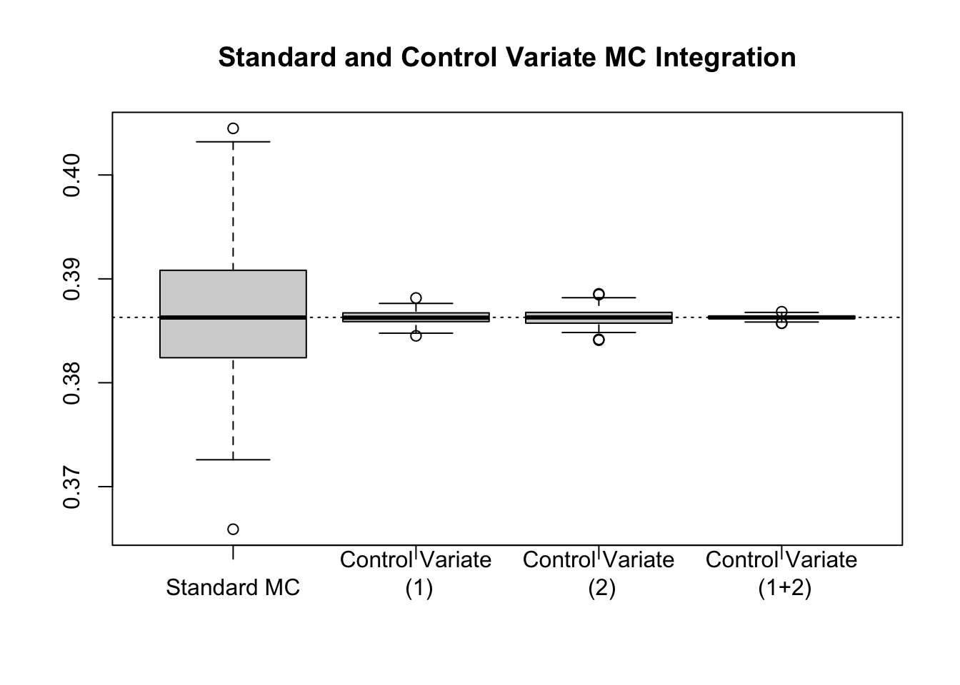
We have seen that when we take an arbitrary integral over an interval, \([a,b]\) we can apply Monte Carlo sampling using a \(\text{Unif}(a,b)\) density. That is, \[\int_{a}^b g(x)dx \approx \frac{b-a}{m}\sum_{i=1}^m g(X_i),\] where \(X_i \sim \text{Unif}(a,b)\). There are at least two issues with this, at least for certain applications. The first is that, as we have seen, this does not work when the limits of integration are infinite. The second is that sampling uniformly from an interval can be quite inefficient to cover the important components of the function, particularly when it is highly non-uniform. To address the first concern we have seen the idea of introducing an alternative density, say \(f(x)\), and rewriting the integral as \[\int_{a}^b g(x)dx = \int_{a}^b \frac{g(x)}{f(x)}f(x)dx = E\left[\frac{g(X)}{f(X)}\right],\] where \(X\) has density \(f(x)\). If we carefully select the density, this can also address the second concern.
We saw an example wherein this method did not yield particularly promising results. In it, we tried to match \(g(x) = \dfrac{1}{1+x^2}\) with \(f(x) = e^{-x}\), since they were defined on the same interval of integration. However, if we consider a plot of the ratio \(g(x)/f(x)\), we can start to see the issue with this choice.
xs <- seq(0, 100, length.out = 10^5)
ys <- exp(xs)/(1 + xs^2)
plot(ys ~ xs, type = 'l', xlab = 'X', ylab = 'g(X)/f(X) (log scale)', log='y', main = 'Ratio of densities')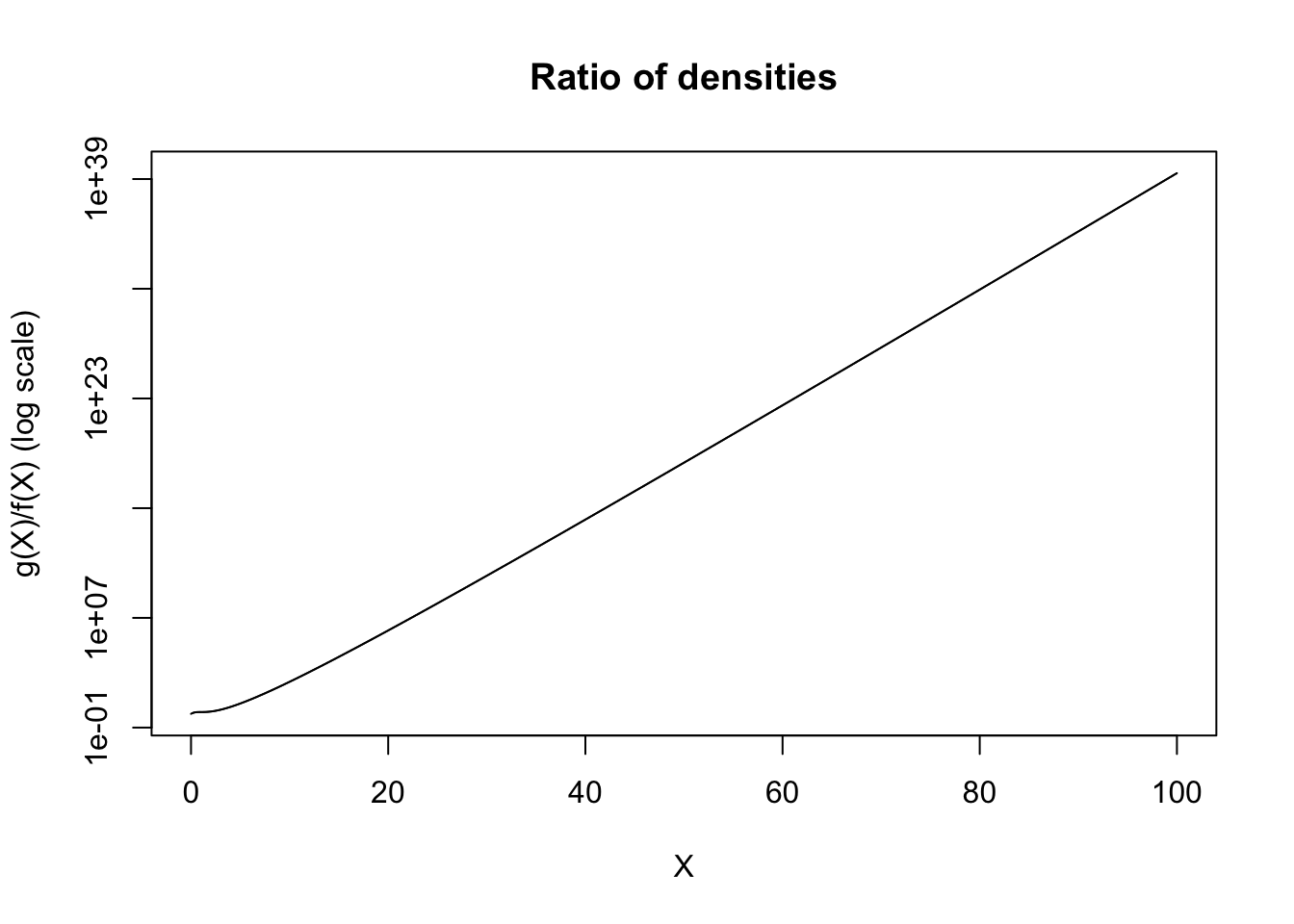
This ratio diverges. If we consider the fact that the performance of the Monte Carlo estimation procedure is predicated upon \(Y = \dfrac{g(X)}{f(X)}\), then if \(Y\) is not a well-behaved random variable, our Monte Carlo estimates will likewise behave poorly. As an extension of this, to have a well performing Monte Carlo estimate, we want \(\text{var}(Y)\) to be as low as possible. In order for \(Y\) to have low variance, we want \(Y\) to be approximately constant, or in other words, for \(g(X) \approx f(X)\) (up to some constants). In fact, in this case, a much more reasonable choice would have been to take \[f(x) = \frac{1}{(1+x)^2},\] which is to say, a (shifted) power law distribution with \(\alpha = 1\) and \(x_m = 1\). In particular, \(X + 1 \sim \text{PL}(1, 1)\). Plotting this ratio gives the following.
xs <- seq(0, 100, length.out = 10^5)
ys <- (1/(1 + xs^2))/(1/(1+xs)^2)
plot(ys ~ xs, type = 'l', xlab = 'X', ylab = 'g(X)/f(X)', main = 'Ratio of densities')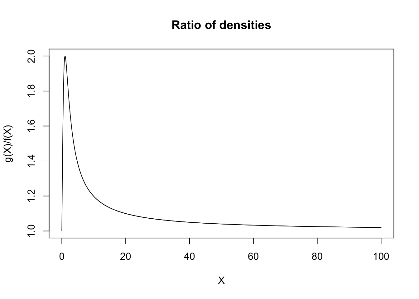
Now generating from a powerlaw distribution can be achieved via inverse-transformation, since the CDF of the random variable is given by \(F(x) = 1 - \left(\frac{x_m}{x}\right)^{\alpha}\), and so \(F^{-1}(x) = \frac{x_m}{(1 - x)^{1/\alpha}}\).
rpowerlaw <- function(n, alpha, xm) {
  xm/((1 - runif(n))^(1/alpha))
}
Then, using this to approach the Monte Carlo problem, we get.
set.seed(31415)

ms <- c(10, 10^2, 10^3, 10^4, 10^5, 10^6, 10^7, 10^8)
fx <- function(x) { ((1+x)^2/(1+x^2)) }

# Compute the averages applied across the various values of 'm'
estimated_vals <- sapply(ms, FUN = function(m) {
  mean(fx(rpowerlaw(m, alpha = 1, xm = 1) - 1))
})

plot(x = ms,
     y = estimated_vals,
     log = "x",
     ylab = "Estimated Value",
     xlab = "Monte Carlo replicates (m; log scale)",
     main = "Monte Carlo Integration with Importance Sampling")
abline(h = pi/2, lty = 3)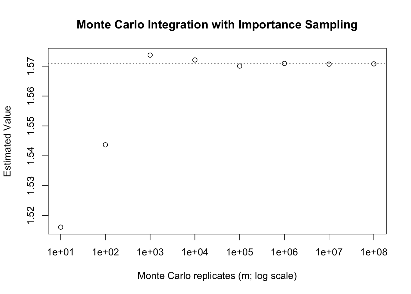
If we consider what we are doing during this process by changing the underlying distribution we are increasing (or decreasing) the frequency with which certain values are sampled. In a sense, we are deciding what areas of the function are important to sample closely, and focusing on those. As a result, we call this importance sampling. Importance sampling can both be used to reduce the variance of a Monte Carlo estimate, or to allow for the computation of an otherwise non-computable integral (for instance, improper integrals).
Suppose, for instance, we want to compute \(E[g(X)]\), where \(g(X)\) is large only when \(g(X) \in A\), for some set \(A\), but where \(P(X\in g^{-1}(A))\) is small. In this case we will generate very few Monte Carlo replicates such that \(g(X) \in A\), and correspondingly, we will underestimate the overall expectation (on average). Instead, it would be better for us to re-weight the integral so that our realizations of the underlying random quantity fall more inline with the important values for the function.
Note that when we discuss \(E[g(X)]\), we have been assuming that we are solving some integral of the form \[\int g(x)f(x)dx,\] where \(f(x)\) is a density function to begin. In importance sampling, we take another density, say \(\phi(x)\), such that \(\phi(x) = 0 \implies g(x)f(x) = 0\),5 and we rewrite this as \[\int g(x)f(x)dx = \int \frac{g(x)f(x)}{\phi(x)}\phi(x)dx = E_{\phi}\left[\frac{g(x)f(x)}{\phi(x)}\right].\] The question is then: which distribution should we use for \(\phi(x)\)?
Per our discussions when motivating importance sampling, it makes sense to try to select \(\phi(x)\) such that the estimator has low variance. In our setup, this would mean taking \(\phi(x) \propto f(x)g(x)\), at least, whenever \(f(x) \geq 0\). It turns out that if \(f(x) < 0\) for any \(x\), then it is best to consider distributions proportional to \(|f(x)|g(x)\). It will generally be impossible to select \(\phi(x) = \kappa|f(x)|g(x)\) for a suitable normalizing constant, \(\kappa\), despite the fact that this choice is optimal. The concern is that, were we able to know what \(\kappa\) would need to be, we would already know the integral \(|f(x)|g(x)\), which in turn suggests that \(f(x)g(x)\) is likely integrable.6
Instead, we use this proportionality as an approximate guide. We know that:
We have seen this rationale applied in the case of trying to integrate \(\frac{1}{1+x^2}\), using a power law density. As an alternative example, consider again the problem of estimating \(\Phi(x)\) in the tails of the density, using the hit-or-miss technique. We saw that while this provided reasonable values when \(x\) was moderate (in the main part of the density), it did not work as well in the tails. The issue here is related to rare events. Suppose that we wish to compute, for instance, \(P(Z \geq 4) = 1 - \Phi(4)\). We know that this probability will be small (far below \(0.01\)) and so even if we generate many, many samples, the chances that we observe any points in this region will be very nearly zero. To get an accurate version of this we would necessitate more draws from the distribution than would be reasonable.
To overcome this, we can use importance sampling. Note that the integral we are approximating is \[\int_{-\infty}^\infty I(t \geq 4)\frac{1}{\sqrt{2\pi}}e^{-t^2/2}dt = \frac{1}{\sqrt{2\pi}}\int_{4}^\infty e^{-t^2/2}dt.\] As a result, we would like a density which is proportional to \(e^{-t^2/2}\) on \([4,\infty)\). One option for this is to recognize that, were we talking about \([0,\infty)\) we could use the exponential distribution (with density \(e^{-x}\)), and so it is quite natural to shift the exponential distribution to begin at \(4\), which is to say that \(X - 4\) has an exponential. This will give a candidate density function of \(\phi(x) = e^{-(x-4)}\) on \([4,\infty)\). Thus we actually solve the integral \[\int_{4}^\infty e^{-t^2/2}dt = \int_{4}^\infty \frac{e^{-t^2/2}}{e^{-(t-4)}}e^{-(t-4)}dt = E_\phi\left[e^{-t^2/2 + t - 4}\right].\] To do so we need to be able to sample from \(\phi(x)\), but note that if we sample \(Y \sim \text{Exp}(1)\) then \(Y + 4\) has the correct distribution: as a result, we can use this simple transformation. Taken together we can estimate \(1 - \Phi(4) \approx 0.00003167\) as follows.
set.seed(31415)

m <- 10^4
fx <- function(x) { exp(-x^2/2 + x - 4) }

# Try the hit-or-miss technique
Z <- rnorm(m)
hom <-  mean(Z >= 4)

# Try the (exponential) importance sampling technique
Y <- rexp(m)
X <- Y + 4
mc.is <- 1/sqrt(2*pi)*mean(fx(X))

c(hom, mc.is)
[1] 0.000000e+00 3.202158e-05Suppose that the function we are trying to integrate, \(g(X)\) varies wildly over different regions of \(X\). In this case we might think to break-up the problem into estimating the integral in a number of different intervals, and then combining these estimators together. Specifically, suppose that we are integrating over \([a,b]\); we can specify a series of points, \(p_1,p_2,\dots,p_{k-1}\) such that \(a = p_1 < p_2 < \cdots < p_{k} < p_{k+1} = b\), and then rewrite the integral of interest as \[\int_{a}^b g(x)dx = \int_{p_2}^{p_2}g(x)dx + \int_{p_2}^{p_3}g(x)dx + \cdots + \int_{p_{k}}^{p_{k+1}} g(x)dx.\] If each of these integrals is more constant, and we use a separate Monte Carlo estimate for each of them, then intuitively this procedure may result in a lower overall variance in the estimator. To make matters concrete, imagine the extreme case of a piece-wise constant model, as in the following figure.
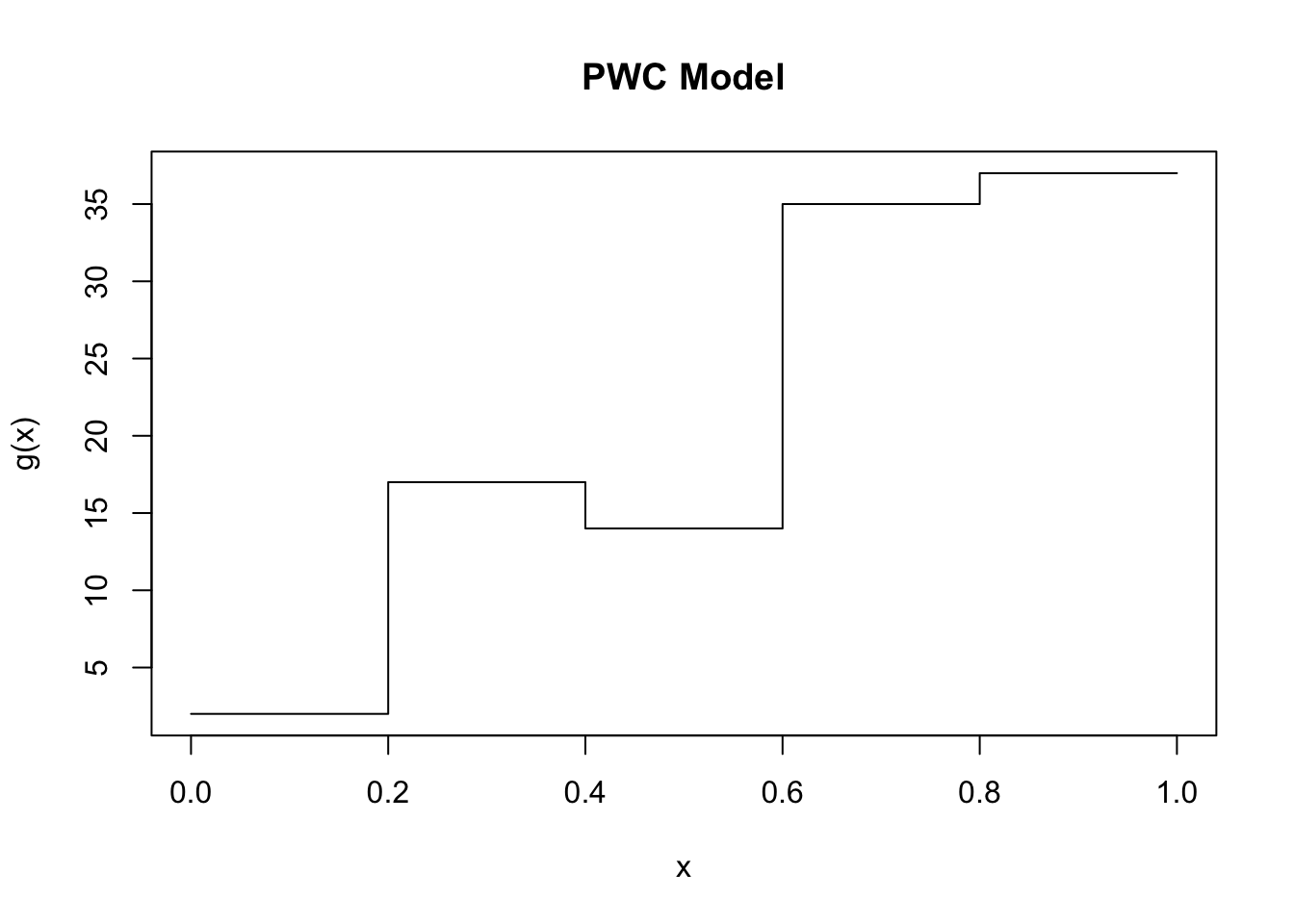
If we wanted to integrate this function and we sample uniformly on \([0,1]\) then there is going to be some large variance in each set of samples as \(g(x)\) ranges from \(\sim 0\) to \(\sim 40\). However, if we cut this into \(k=5\) components, equally throughout, then on each of those components \(g(x)\) has variance \(0\). Adding together \(5\) independent quantities, each with variance \(0\) maintains a result of variance \(0\). Even when the function is not nearly constant, if it is well-behaved (say, continuous) then dividing the interval of integration into sensible chunks will likely have the effect of reducing the variance. This presents an idea for improving the results of our Monte Carlo methods, namely stratified sampling. We first divide the interval into several strata, then perform Monte Carlo integration within each strata independently. If we use \(k\) strata, we use \(m_1,m_2,\dots,m_k\) samples from each of them, resulting in \(m=\sum_{i=1}^k m_i\). If we sample within each strata uniformly, then it is sensible to take \[\widehat{\theta}^{(k)} = \frac{1}{k}\sum_{i=1}^k \widehat{\theta}_i.\] However, if our initial sampling is non-uniform, then it is perhaps more reasonable to use the density \(f_j(u) = f(u|p_{j} \leq U \leq p_{j+1}) = \frac{f(u)}{P(p_j \leq U \leq p_{j+1})}\). Then each strata is weighted by \(P(p_j \leq U \leq p_{j+1}) = P_j\) in the final summation.
Suppose that we divide up our total points proportional to the probability of falling in the strata, which is to say \(m_i = P_im\), and have each interval independent of the next. Take \(\text{var}(g(X))\) to be \(\sigma_i^2\) on the \(i\)th strata. Then, \[\text{var}(\widehat{\theta}^{(k)}) = \text{var}\left(\sum_{i=1}^kP_i\widehat{\theta}_i\right) = \sum_{i=1}^k P_i^2\frac{\sigma_i^2}{P_im} = \frac{1}{m}\sum_{i=1}^kP_i\sigma_i^2.\] Now, we can consider the variance of the standard estimator, which is given by \[\text{var}(\widehat{\theta}) = \frac{1}{m}\text{var}(g(U)) = \frac{1}{m}\left[E[\text{var}(g(U)|h(U))] + \text{var}(E[g(U)|h(U)])\right],\] for any \(h(U)\). If we consider \(h(U) = j\) if \(p_{j} \leq U \leq p_{j+1}\), for \(j=1,\dots,k\), then we can get \[E[\text{var}(g(U)|h(U))] = \sum_{i=1}^k P_i\sigma_i^2 = m\cdot\text{var}(\widehat{\theta}^{(k)}).\] Moreover, \[\text{var}(E[g(U)|h(U)]) = \text{var}(\theta_{h(U)}) = \sum_{i=1}^k P_i(\theta_j - \theta)^2 \geq 0.\]
Thus, taken together we have \[\text{var}(\widehat{\theta}) = \frac{1}{m}\sum_{i=1}^kP_i(\sigma_i^2 + (\theta_i - \theta)^2).\] Thus the stratified estimator (with proportional allocation) will have lower variance in this setting. Generally, we can improve over proportion allocation by using \(m_i \propto P_im\sigma_i\), however, this relies on having the true standard deviations of each interval (a fairly strong assumption). Not only will we typically use proportional allocation, in practice, we will most commonly apply stratified sampling by dividing the region of integration into equal parts, and then equally weighting each part (computing the integral within each as is required).
Suppose that we wish to integrate \[\int_{0}^1 \frac{e^{-x}}{1+x^2}dx,\] using uniform draws on \([0,1]\). We can stratify this to see the effect of stratification across various values of \(k\). We will use equal weighting and proportional allocation.
repeat_experiments <- 200

m <- 10000
gx <- function(x) { exp(-x) / (1 + x^2) }
ks <- c(1, 2, 4, 8, 16, 50) # Number of Strata
rs <- m / ks # Number of replicates per strata

set.seed(31415)

results <- matrix(0,
                  nrow = repeat_experiments,
                  ncol = length(ks))

for(ii in 1:repeat_experiments) {
  for(idx in 1:length(ks)) {
    k <- ks[idx]
    results[ii, idx] <- mean(sapply(seq(0,
                                        1,
                                        length.out = k+1)[1:k],
                                    function(lb) {
      mean(gx(runif(rs[idx], min = lb, max = lb + 1/k)))
    }))
  }
}

colnames(results) <- ks
boxplot(results, xlab ='Number of Intervals')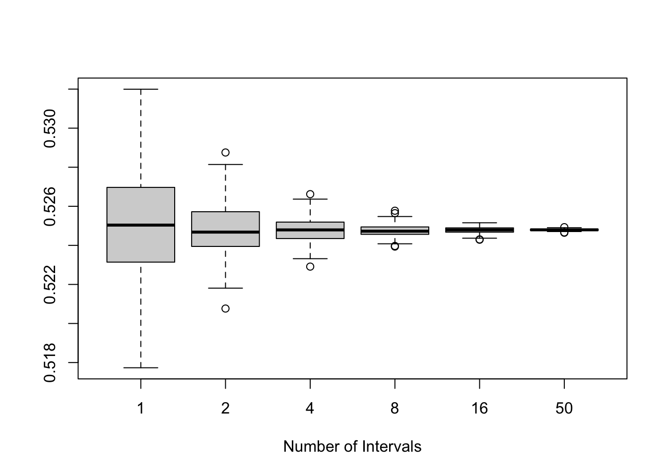
In practice for the integrals that we solved in these notes, using Monte Carlo techniques would be less than ideal. The concern is that generally speaking, Monte Carlo techniques trade-in computational efficiency to achieve ease of use. The ideas are (comparatively) straightforward, and the cost to pay for this is that computing these integrals can take a very long, particularly when compared with other numerical approximation techniques. However, Monte Carlo techniques have a very intriguing property, which makes them increasingly useful in certain contexts: the absolute error of the estimation is on the order of \(\dfrac{1}{\sqrt{m}}\). That is, we expect that the difference between our estimated value and the truth is going to be some constant times by \(m^{-1/2}\). The intriguing part about this result is that it does not depend on the dimension of the integral.
We have been assuming that \(d=1\) throughout the talk, but in practical applications (say from physics, engineering, or finance) the integrals of interest will often be high dimensional (say \(3-12\) in physics, and plenty more in both engineering and finance). The absolute error in estimating integrals in larger dimensions will remain on the order of \(m^{-1/2}\), so long as the functions are nicely behaved. In contrast, numerical integration techniques scale exponentially in the dimension, meaning that if \(m=1000\) samples is enough for \(d=1\) then \(d=4\) requires \(\sim 1000^4 = 1,000,000,000,000\) samples for the same absolute error.7 As a result, as soon as the dimension scales even slightly, it rapidly becomes more computationally efficient to use Monte Carlo techniques than to use numerical techniques (and indeed, these techniques see wider appeal in higher dimensional contexts).
There are some hurdles to watch out for in high dimensions, some of which can be resolved via the use of techniques which have been discussed (such as importance sampling), some of which can be resolved via the use of techniques beyond our discussions (such as Quasi-Monte Carlo techniques), and some of which remain unresolved. For one, despite the fact that the absolute error does not grow with dimension, the relative error might. The issue is that in higher dimensions the number of points that fall into the relevant space become sparser and sparser, and as a result, we run into issues similar to those seen with importance sampling. In high dimensions importance sampling can resolve this, however, it may not always be easy to find a density to use in the importance sampling procedure. Moreover, while the error is on the order of \(m^{-1/2}\), there is a constant that multiplies this error: this constant may be dependent on the dimension of the problem, and may be non-negligible compared to \(m^{-1/2}\) for feasible values of \(m\). That is, we know that as \(m\to\infty\) the constant is rendered irrelevant, however, for any finite \(m\) the constant may be large. To make the point concrete, suppose that we know that the absolute error is given exactly by \[\text{Error} = \frac{10^{4d}}{\sqrt{m}}.\] As \(m\to\infty\), in any dimension, this error goes to zero (and does so at a rate of \(m^{-1/2}\)). However, suppose that we compare \(d=1\) to \(d = 100\) and that a suitable error for the application is \(1\). In this case we require \(m = 10^8\) in the \(1D\) case. This is a lot of samples, but it is likely manageable (as we have seen in some of these examples). In the \(d = 100\) case, we require \(m = 10^{800}\), a number so large so as to be totally infeasible. This is an extreme example, but it illustrates the point that sometimes an asymptotic analysis is insufficient for our goals.
Still, Monte Carlo techniques remain among the most feasible techniques whenever we need to numerically approximate high dimensional integrals. For this reason they form a critical component of many applied fields, even ones which seem to have very little to do (on the surface) with statistical reasoning.
A much better choice would have been to recognize that \(\frac{1}{\pi(1 + x^2)}\) is the Cauchy distribution density function, and thus this integral is actually fairly straightforward to compute directly.↩︎
You can also divide by \(m-1\), though, ultimately it will not make much of a difference.↩︎
See for instance, the course textbook pp. 156-157↩︎
If you have taken linear regression, it is worth considering why the \(R^2\) is equivalent to the percent reduction in variance.↩︎
This assumption is to ensure that division by \(\phi(x)\) does not pose any concerns for the integration.↩︎
This is not necessarily true, but will be in many cases.↩︎
Note, the absolute error for numerical methods depends on which numerical method is used, and also often depends on the precision you want to specify, so the scaling may be slightly more complicated than this, but this gives a good “rule of thumb”.↩︎