# Specify Parameter Values for the Simulation
n <- 1000             # Sample Size
theta <- 10           # True Parameter Value
alphas <- c(1,2,3,4)  # Nuisance Parameter Values
repeats <- 1000       # How many times to repeat the experiment
                      # Some condition that you are testing against.
exp_cond <- 1:10      # This may be theta, or n, or alphas, or something else
                      # entirely.

# Specify a Matrix to Hold the results in
# Likely one row per run, and one column per estimated value
# Pre-allocating allows for more efficient simulation runs
results <- matrix(0, nrow = repeats, ncol = length(exp_cond))

set.seed(31415) # Seed is *incredibly* important for simulations.

# Start the loop for simulation runs
for(ii in 1:repeats) {
  # Start a loop for the experiment conditions
  for(jj in 1:length(exp_conds)) {
    # Generate Data for the particular condition
    my_data <- dataGenerate(n, theta, alphas, exp_cond[jj])

    # Apply the Methods to the Generated Data
    my_theta <- myMethod(my_data)

    # Store the Result
    results[ii, jj] <- my_theta
  }
}

# Display the Results in a Useful Manner
boxplot(results)Monte Carlo Simulation Techniques
Experiments in Statistical Research
Simulation Studies
When we envision doing research in any of the physical sciences, we likely imagine lab or field experiments. Even quantitative research in the social sciences tends to be driven by experimental findings. Experiments are useful for learning about the world owing to the control that we have over the environment. We know the behaviour of all conditions which our external to those of interest, and because of this, any findings we observe can be attributed to the experimental conditions. While statistics research differs in meaningful ways from research in other fields, we also rely heavily on experiments to conduct effective research.
Suppose you are developing a new estimator for a particular quantity that you wish to apply on real-world data. In our classes we have seen that we can often determine theoretical properties of estimators (showing that they are theoretically unbiased, that their variance is a certain value, etc.). This theory, however, is frequently predicated upon sets of assumptions about the underlying data. Sometimes the assumption is that the sample size is growing large enough to be considered infinite. Sometimes the assumptions relate to the underlying distribution of the data. No matter the particular nature, theory tends to be predicated upon a set of assumptions in order to remain valid. However, in practice, we are never going to have infinite data available, and we are not likely to know the exact distribution of the population. How can we be sure that the techniques are going to perform as expected?
The fundamental issue we face is that, when confronted with the real world, statistical estimation is influenced by myriad factors outside of our control. These factors can undermine theoretical results, making the estimators unsuited to the task. The hard part is, however, that from the point of view of someone conducting an analysis, there is no way to tell whether the estimator performed well on a particular data set or not. If we do not know the true value of \(\theta\), it is challenging to know whether \(\widehat{\theta}\) is a good representation of it. To overcome this we use experimental techniques, specifically in the form of simulation studies.
Monte Carlo Techniques
In statistics, Monte Carlo techniques refer to any class of techniques which rely on the repeated generation of (pseudo) random values in order to understand an underlying phenomenon. Monte Carlo methods are used for many different tasks, but from a Statisticians perspective, the most common reason for application is for simulation experiments.
Simulation Experiments: Overview
The process of running a simulation experiment relies on a three-step procedure.
- Determine what experimental conditions are desired.
- Setup the probability models to test the desired experimental conditions.
- Summarize and communicate the experimental results.
The choices made at each step are going to be subjective, based on the underlying subject matter. For instance, you may wish to understand how sample size impacts the performance of a method which is asymptotically unbiased. In this case perhaps you choose various relevant sample sizes, \(n\in\{10,100,1000,10000\}\) and then generate data according to the theoretically optimal probability model for the given technique. You can then perform the estimation on each of these data sets, and repeat these results \(1000\) times for each \(n\). A set of box plots can then summarize the techniques, along with a description of the performance based on the findings. In this example we are interested in the impact of the sample size, and so we keep the distribution to be what we understand will perform well. Perhaps, instead, we are interested in how deviations from normality impact the performance of the technique. In this case, you may choose to fix \(n=1000000\) (or some other suitably large value) and then consider some sequence of distributions, say \(\{t_2, t_4, t_{10}, t_{15}, t_{25}, t_{50}, t_{100}, N(0,1)\}\) over which your method can be tested. Once again, the results could then be repeated many times over, and the results could be summarized in a suitable graphic or table. Here it is deviations from normality we are interested in, and so we keep \(n\) to be large.
Simulations are particularly useful for testing small sample performance of techniques, or the robustness to assumptions made in the theoretical development. Modern statistics papers, even those which are theoretically heavy, almost all report simulation experiment results validating their techniques. If you open any of these papers there is likely to be a section of the paper entitled something like “Simulations” or “Experiments” or “Examples”, in which you will find the result of Monte Carlo experiments run on the methods. These sections will often indicate the shortcomings of the techniques, or display the range of settings in which the techniques are most appropriate. They are a very useful place to scan while reading through a paper. In fact, some modern statistical papers are formulated almost entirely through simulation results.
Simulation Experiments: General Format
To program a simulation in R, the following structure will typically be used.
The details of the simulation will need to be filled-in for any specific use case. However, this shows the general process of first establishing what the experiment to perform will be, then translating this to a data generation mechanism and repeating that process many times over, before finally outputting the results. Typically, several distinct simulations will be performed testing various performance characteristics of the method. If the simulation results are positive, or are positive under certain relaxed assumptions, and there is theoretical support for the application of a particular technique then this likely provides sufficient justification to actually start applying the technique on real-world data sets.
Uses for Simulation Experiments
We present the simulation techniques as being particularly useful for testing the viability of different methods under violations to the assumptions that drove the theory. It is also possible to use the same sets of techniques to assess methods in ways which are challenging to do theoretically. A common example of this is in the assessment of hypothesis tests. While we typically design hypothesis test procedures to control the Type I error rate (\(\alpha\)), we like to assess hypothesis tests via their propensity to make Type I or Type II errors. More often than discussing the type II error rate, we talk about the power of a hypothesis test, which is the probability that we reject the null hypothesis, correctly. This can be an incredibly challenging quantity to compute analytically, however, via simulation it is fairly easy to approximate: we simply generate data where the null hypothesis is in fact false, and then determine the proportion of time that the procedure makes the correct conclusion in the test.
Simulations can also be useful to estimate the variance of estimators, or indeed to approximate the finite-sample sampling distribution of the estimator. This can be challenging to compute for small \(n\), but can be done rather effectively through repeated experimental runs. This type of procedure is useful for the development of confidence intervals, or other uncertainty quantification procedures. If you have a procedure for generating a confidence interval for an estimator of interest, simulations can be useful to test the empirical coverage of this interval. If you perform the procedure many times over, in what proportion of these simulated experiments does the confidence interval contain the truth (a question which you can answer since in these settings you know the truth!)?
A final example use for Monte Carlo experiments1 is for assessing the performance of a predictive model. While certain types of predictive models make theoretical guarantees on the predictive performance of the model, it is often challenging to determine these analytically. With simulation experiments we can readily generate many out-of-sample data points on which predictions can be performed, and the accuracy of the model can be determined. This also allows for the testing of predictive models under distributional shift (a common concern in practice), or assessing the ability to capture prediction uncertainty (through, for instance, prediction intervals).
Alternative Experimental Procedures
Sometimes it can be challenging to know precisely what data generation mechanism should be used. In these cases the method may be more designed to work with particular data, or data following a particular layout, but similar testing is still desired. In these cases it may be possible to perform the experiment using real-world data with sufficient access to the correct answers. For instance, suppose that you have developed a prediction technique. You may wish to apply this technique to make predictions moving forward. If you have historical data for the phenomenon you are attempting to predict, this can serve as a particularly relevant data source to test the method on. Because the data are historical you have the correct answers, and so this process can be performed again where instead of pseudo random data, the real data are used.
If you take this path it is critically important to not use the data that you are “training” your model with to “test” your model. You need to hold out some of the data which will serve as the data to test the performance, and then train your model on the remaining data. The data that you held out will then act as though it is future data your predictions can actually be applied to. This framing of experiments is quite popular, particularly in machine learning work and computer science more broadly, where prediction is prevalent and synthetic data may be insufficiently complex. Despite these benefits, there are some notable drawbacks to the technique. The first is that it is challenging to repeat this many times over, which does not lend itself well to understanding the variability of the methods. The second is that, because the data are not synthetic, and because you have only one source of data, positive performance of a model may not reflect truly positive results and may instead be the result of sampling variability (same with negative results). These trade-offs need to be balanced in practice.
Example Projects
In what follows we consider several different simulation experiments, for a variety of scenarios, to better demonstrate the underlying ideas.
Convergence of the Sample Mean
set.seed(314159)

# We wish to test how the sample mean converges over increasing
# sample size. Particularly we want to see this behaviour for
# heavy-tailed distributions. [t(3), say]

ns <- c(5, 10, 15, 30, 50, 100, 1000)
repeats <- 1000
results <- matrix(0, nrow = repeats, ncol = length(ns))

for (ii in 1:repeats) {
  for (jj in 1:length(ns)) {
    n <- ns[jj] # Grab the sample size

    results[ii, jj] <- mean(rt(n, df = 3))
  }
}

# Plot a Boxplot
colnames(results) <- ns

boxplot(results,
        xlab = "Sample Size",
        main = "Boxplots of Convergence of Sample Mean Over Various
        Sample Sizes")
abline(h = 0, lty = 3)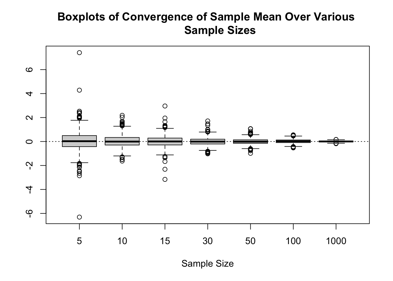
We could also report the MSE for each of these values as:
| Sample Size | MSE |
|---|---|
| 5 | 0.641 |
| 10 | 0.244 |
| 15 | 0.214 |
| 30 | 0.095 |
| 50 | 0.057 |
| 100 | 0.028 |
| 1000 | 0.003 |
Bias in the Estimation of Sample Variances
We learn in introductory statistics courses that \(\frac{1}{n-1}\sum_{i=1}^n (X_i - \overline{X})^2\) is preferable for the sample variance estimator as it is unbiased. We can assess how the bias is impacted by the constant that we choose (and also the performance) over various values for the sample size. We will compare estimation with \((n-1)^{-1}, n^{-1}\) and \((n+1)^{-1}\).
set.seed(314159)

# Set the sample sizes
ns <- c(5, 10, 15, 20, 30, 50, 100)
repeats <- 1000
sq_results <- matrix(0, nrow = repeats, ncol = length(ns))

for (ii in 1:repeats) {
  for (jj in 1:length(ns)) {
    n <- ns[jj] # Grab the sample size

    # Generate a Sample
    X <- rnorm(n, mean = 0, sd = 2)

    # Store the Sum of Squared Results
    # Can be normalized via n afterwards.
    sq_results[ii, jj] <- sum((X - mean(X))^2)
  }
}

# Produce the Actual Results
db_n_m_1 <- t(t(sq_results) / (ns - 1))
db_n <- t(t(sq_results) / (ns))
db_n_p_1 <- t(t(sq_results) / (ns + 1))

# Create an MSE table: true value is 4
results_df <- data.frame(
  "Sample Size" = ns,
  "n - 1" = colMeans((db_n_m_1 - 4)^2),
  "n" = colMeans((db_n - 4)^2),
  "n + 1" = colMeans((db_n_p_1 - 4)^2),
  check.names = FALSE
)

# Produce Quarto table
knitr::kable(results_df, align = "c", row.names = FALSE, digits = 4)| Sample Size | n - 1 | n | n + 1 |
|---|---|---|---|
| 5 | 7.6229 | 5.3584 | 4.9431 |
| 10 | 3.4129 | 2.9091 | 2.7882 |
| 15 | 2.2889 | 2.0939 | 2.0533 |
| 20 | 1.6340 | 1.5153 | 1.4838 |
| 30 | 1.0566 | 1.0028 | 0.9869 |
| 50 | 0.7032 | 0.6851 | 0.6803 |
| 100 | 0.2931 | 0.2883 | 0.2867 |
# Create a mean bias table: true value is 4
results_df2 <- data.frame(
  "Sample Size" = ns,
  "n - 1" = colMeans((db_n_m_1 - 4)),
  "n" = colMeans((db_n - 4)),
  "n + 1" = colMeans((db_n_p_1 - 4)),
  check.names = FALSE
)

# Produce Quarto table
knitr::kable(results_df2, align = "c", row.names = FALSE, digits = 4)| Sample Size | n - 1 | n | n + 1 |
|---|---|---|---|
| 5 | 0.1252 | -0.6998 | -1.2498 |
| 10 | 0.0214 | -0.3808 | -0.7098 |
| 15 | -0.0581 | -0.3209 | -0.5508 |
| 20 | -0.0015 | -0.2015 | -0.3823 |
| 30 | 0.0091 | -0.1245 | -0.2496 |
| 50 | -0.0219 | -0.1014 | -0.1779 |
| 100 | 0.0078 | -0.0323 | -0.0716 |
Power of a \(t\)-Test
Suppose that we wish to test \(H_0: \mu = \mu_0\) versus the alternative \(H_1: \mu \neq \mu_0\). Moreover, suppose that the null hypothesis is false. We might be interested in the probability that we correctly reject the null hypothesis in this case, which is to say the power of the test. To get an estimate of the power we want to use a range of values. So, suppose that we have \(X \sim N(\mu,4)\) as our true distribution. We will consider a range of \(\mu\), say from \([-1, 1]\) and have our test value be \(0\) all the time. We will keep the sample size fixed (at \(n=1000\)).
set.seed(314159)

# Set the sample sizes
n <- 1000
mus <- seq(-1, 1, length.out = 501) # Run 501 values for the mean!
repeats <- 5000
results <- matrix(0, nrow = repeats, ncol = length(mus))

for (ii in 1:repeats) {
  for (jj in 1:length(mus)) {
    mu <- mus[jj] # Grab the sample size

    # Generate a Sample
    X <- rnorm(n, mean = mu, sd = 2)

    # Check if the p <= 0.05 (e.g. we reject H0).
    results[ii, jj] <- t.test(X)$p.value <= 0.05
  }
}

# Summarize the Results
empirical_power <- colMeans(results)

plot(empirical_power ~ mus,
     main = "Empirical Probability of Rejecting the Null \n t-test of H0: mu = 0",
     xlab = expression("True" ~ mu),
     ylab = expression(pi[n](mu)),
     type = 'l')
abline(h = 0.05, lty = 3, col = 'red')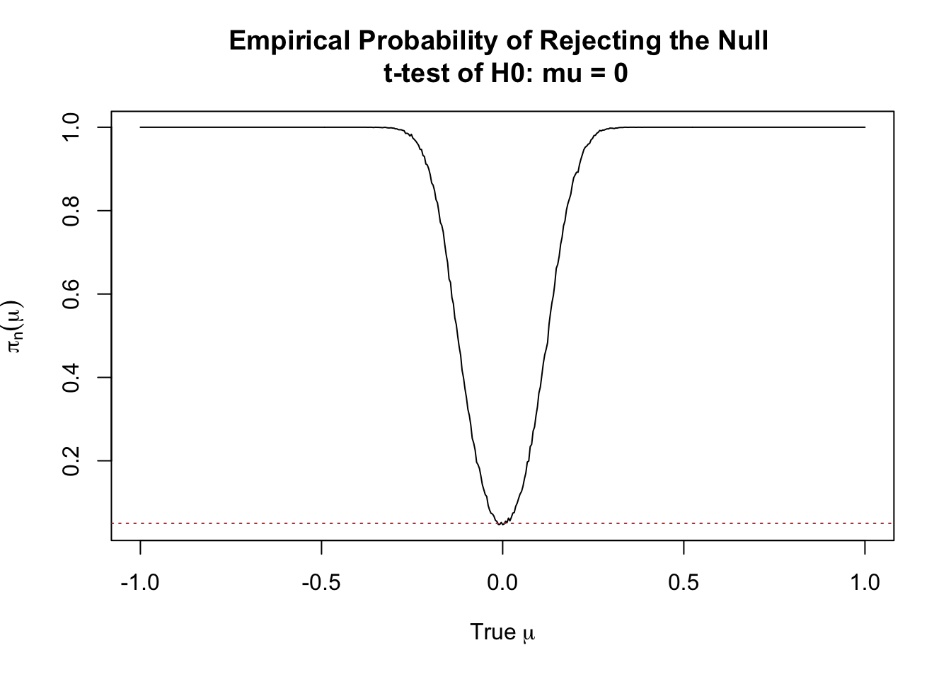
Coverage of a Confidence Interval for a Mean
Confidence intervals for the sample mean can be formed using the CLT to approximate the sampling distribution, even when the sample variance is unknown. The idea with a confidence interval is that if the process is repeated over and over to generate the confidence interval, then with probability \(1-\alpha\), the true value will be contained in the formed interval. Thus, if we form \(95\%\) confidence intervals for the mean, then we will expect that in approximately \(95\%\) of cases the process will capture the truth.
set.seed(314159)

# Set the sample size
n <- 9
mu <- 3
repeats <- 5000

# Run the analysis with the normal approximation and using
# the more correct 't' distribution, for n
results_norm <- matrix(0, nrow = repeats, ncol = 3)
results_t <- matrix(0, nrow = repeats, ncol = 3)

for (ii in 1:repeats) {
  # Generate a Sample
  X <- rnorm(n, mean = mu, sd = 2)

  xbar <- mean(X)
  sd <- sd(X)
  se <- sd/sqrt(n)

  upper_N <- xbar + se * qnorm(0.975)
  lower_N <- xbar - se * qnorm(0.975)
  upper_t <- xbar + se * qt(0.975, df = n-1)
  lower_t <- xbar - se * qt(0.975, df = n-1)

  results_norm[ii, ] <- c(lower_N, upper_N, upper_N >= mu && lower_N <= mu)
  results_t[ii, ] <- c(lower_t, upper_t, upper_t >= mu && lower_t <= mu)
}

# Summarize the Results
# Plot the first 100 and then compute means on the reaminders
x_vals <- 1:repeats
y_start_t <- results_t[1:100,1]
y_end_t <- results_t[1:100,2]
col_t <- ifelse(results_t[1:100,3], "blue", "red")
y_start_norm <- results_norm[1:100,1]
y_end_norm <- results_norm[1:100,2]
col_norm <- ifelse(results_norm[1:100,3], "blue", "red")

plot(NULL,
     ylim = c(min(results_t[,1]), max(results_t[,2])),
     xlim = c(1, 100),
     main = "Coverage Plot: t Based CIs",
     xlab = "Experiment #",
     ylab = expression("Confidence Interval for"~mu))
segments(x0 = x_vals,
         x1 = x_vals,
         y0 = y_start_t,
         y1 = y_end_t,
         col = col_t,
         lwd = 1.4)
abline(h = mu, lty = 2)
plot(NULL,
     ylim = c(min(results_norm[,1]), max(results_norm[,2])),
     xlim = c(1, 100),
     main = "Coverage Plot: Normal Based CIs",
     xlab = "Experiment #",
     ylab = expression("Confidence Interval for"~mu))
segments(x0 = x_vals,
         x1 = x_vals,
         y0 = y_start_norm,
         y1 = y_end_norm,
         col = col_norm,
         lwd = 1.4)
abline(h = mu, lty = 2)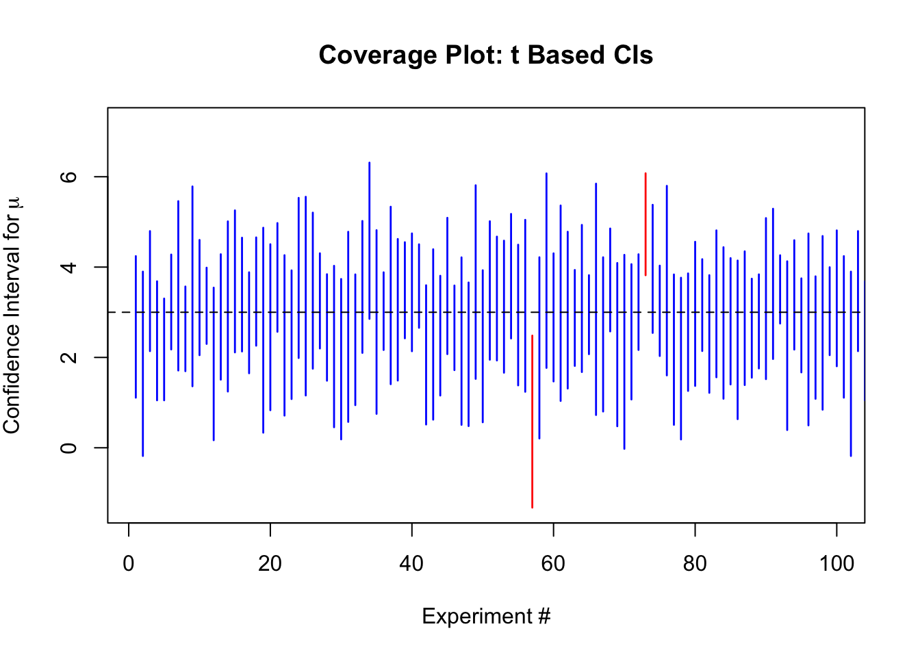
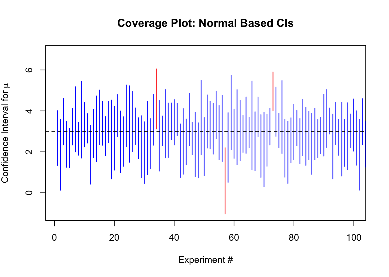
The empirical coverage for the \(t\) based intervals is 95.46%, and for the normal based intervals is 91.62%.
Footnotes
Many more such uses exist in practice, but listing them all is an endless endeavour.↩︎