Markov Chain Monte Carlo
Introduction
In our statistical computing course, we have discussed a class of techniques known as Monte Carlo methods. A particular topic of Monte Carlo methods that we considered was Monte Carlo integration. This document will build upon that framework of integration to present a related type of procedures known as Markov Chain Monte Carlo (MCMC) methods. This broad range of techniques is especially useful in cases where regular Monte Carlo integration fails, and MCMC has found itself numerous applications in a wide variety of fields. We begin by introducing the topic of stochastic processes, which will be a precursor to Markov Chains. The section on Markov Chains is quite long, since there is a large quantity of background knowledge required to understand how Markov Chains become incredibly useful in MCMC. After exploring the topic of Markov Chains, we will dive into the culmination of this document, Markov Chain Monte Carlo integration.
Stochastic Processes
A stochastic process is a random process in which we have a sequence of random variables. It is a set \({\{X_t\:|\:t\in{T}\}}\) where the \(X_t\)’s are random variables indexed by the set \(T\). We call the set \({\{X_t\:|\:t\in{T}\}}\) the state space of the stochastic process, since it is useful to think of each \(X_t\) as a possible state of a given system. For example, we can think of the \(X_t\)’s as denoting, at a certain time \(t\), the number of customers waiting in line at the cashier in a store: over time, the number of customers waiting in line changes randomly, and so maybe at time t=0 we have \(X_0=3\) customers, and then at the next time step \(t=1\) we may have \(X_1=4\) customers. The state space can be a discrete or continuous set, and it can be finite or infinite. Same goes for the index set \(T\): it can be discrete or continuous, finite or infinite. Note that in many situations (though this doesn’t have to be the case), the index set \(T\) is thought of as representing time (in either continuous time that or discrete time).
Markov Chains
Markov Chains are a certain type of stochastic process. They are a sequence of random variables \({\{X_t\:|\:t\in{T}\}}\) indexed by a set \(T\) that satisfy a certain property (which will be discussed shortly). In this section, we focus on the theory of discrete, finite state space and discrete, finite time Markov Chains. However, infinite state space Markov Chains will come into play when we learn about Markov Chain Monte Carlo methods.
Suppose our state space is \({\{X_t\:|\:t\in{T}\}}\), where \(X_t\in\{1,\:2,\:3,...,\:m\}\) and where \(T=\{0,\:1,\:2,...,\:n\}\). We can think of the subscript \(t\) as representing the current point in time, and that increasing \(t\) means we are jumping ahead in time by discrete units. As discussed before, it is useful to think of each possibility \(X_t\) in the state space as representing a possible state of a certain system. In our case, we have \(m\) different possible states in our system, ranging from \(1\) to \(m\), and the sequence of random variables \(X_t\) can be thought of as jumping from one state to the next as we increase time.
These transitions from state to state occur with certain probabilities. The probability of jumping from state \(i\) to state \(j\) is denoted by \(p_{ij}\). This is what is referred to as a one-step transition probability, i.e., the probability that our system goes from state \(i\) to state \(j\) as we increment the index \(t\) by one. Written formulaically, \(p_{ij}=P[\,X_{t+1}=j\:|\:X_t=i\,]\). The goal of constructing and using a Markov Chain is to understand probabilistically how the system of interest will evolve over time.
The defining feature of a Markov Chain that distinguishes it from other stochastic processes is the following property, called the Markov Property or the Markov Assumption:
\[ p_{ij}=P[\,X_{t+1}=j\:|\:X_t=i\,]=P[\,X_{t+1}=j\:|\:X_t=i,\:X_{t-1}=i_{t-1},\:X_{t-2}=i_{t-2},...,\:X_0=i_0\,]. \]
This property guarantees that the probability of transitioning from state \(i\) to state \(j\) does not depend on the transitions that have occurred in the past. Instead, the transition probabilities only depend on which state is occupied in the present. Thus, there is a one-step dependence between the random variables in the Markov Chain.
As an example, consider the following. Suppose that the probability of transitioning from state \(i\) to state \(j\) were \(0.3\), and suppose that this transition has just occurred. Now, imagine that the chain continues to jump from state to state as time progresses, finally returning some time later to state \(i\). Even though many steps may have occurred since the last time the chain was at state \(i\), the probability of it transitioning from \(i\) to \(j\) remains \(0.3\). This is the essential idea of the Markov Property.
The following steps illustrate how to construct a Markov Chain:
Specify the possible states of the model;
Identify the possible transitions between states;
Indicate the transition probabilities.
When determining the specifics of a Markov Chain, it is important to correctly specify the above components of the chain in order to make it satisfy the Markov Property. Incorrectly specifying the chain can cause it to not have the desired properties.
An Example of a Markov Chain
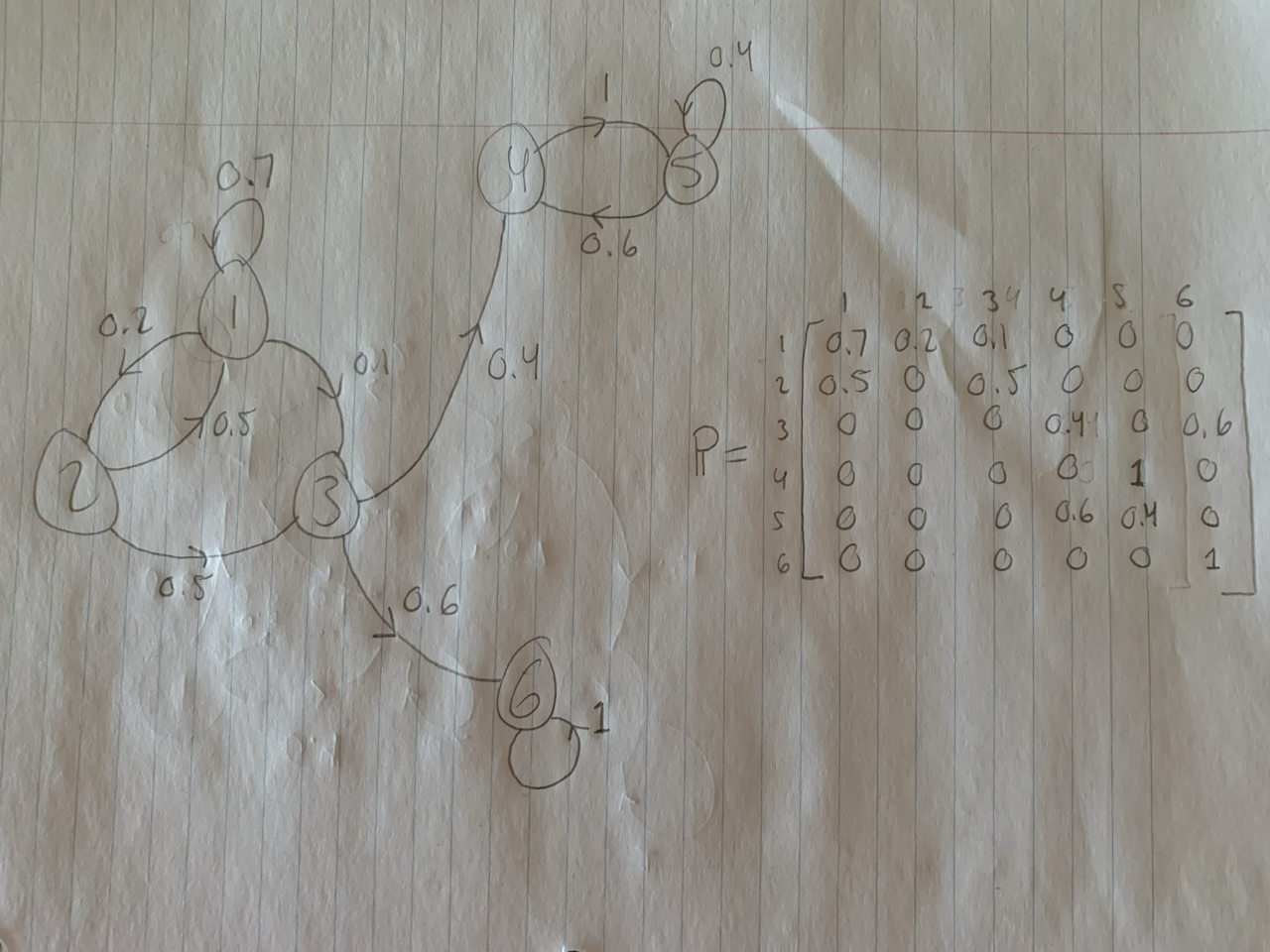
Before we investigate certain features and properties of Markov Chains, let us explore an example of one. The figure below illustrates a simple example of a Markov Chain. In this figure, the numbered circles represent the different possible states of the system. An arrow pointing from a certain state \(i\) to a certain state \(j\) is labelled with the transition probability \(p_{ij}\). For example, there is an arrow pointing from state \(3\) to state \(6\), meaning there is a possible one-step transition from \(3\) to \(6\), and the number \(0.6\) next to that arrow indicates that this transition has probability \(0.6\) of occurring. Note that states can transition to themselves, which is indicated by loops in the diagram.
Another thing to note is that although certain states are not directly connected (for example, state \(1\) is not directly connected to state \(4\)), the system can sometimes still move between these states; it may simply take more than one step (for example, to get from state \(1\) to state \(4\), the system could follow \(1\rightarrow1\rightarrow2\rightarrow3\rightarrow4\), or \(1\rightarrow3\rightarrow4\)). However, it can also be the case that states cannot “communicate” with each other at all. This occurs between states \(6\) and \(5\) in the illustration below.
A final remark about this example is the matrix located on the right-hand side of the page. This matrix \(\mathbb{P}\) is called the transition matrix (this matrix exists for any finite state space Markov Chain). Its rows and columns are indexed by the different states of the system, as shown in the picture. The \((i,j)\)-entry of the transition matrix denotes the transition probability \(p_{ij}\).
k-Step Transitions
Building on the notion of one-step transition probabilities, we can define k-step transition probabilities. The k-step transition probability \(p_{ij}^{(k)}\) denotes the probability of going from state \(i\) to state \(j\) in exactly \(k\) steps (there can be many such paths), that is, \(p_{ij}^{(k)}=P[\,X_k=j\:|\:X_0=i\,]\). It turns out that \(p_{ij}^{(k)}\) is simply the \((i,j)\)-entry of \(\mathbb{P}^k\), where \(\mathbb{P}^k\) is the \(k^{th}\) power of the transition matrix \(\mathbb{P}\).
Our next consideration will be on what the probability of being at a certain state in the system will be. That is, over the course of running the chain, what is the probability of being at state \(i\)? We have seen the notion of a k-step transition probability with a given starting point, but what if the starting point is random?
To answer this question, we can resort back to the regular k-step transition probabilities in which the starting point is fixed. For any given \(i\), \(p_{ij}^{(k)}\) is the probability that, starting from state \(i\), we arrive at state \(j\) in \(k\) steps. Now, if we randomize the starting point, there is a probability \(P[\,X_0=i\,]\cdot{p_{ij}^{(k)}}\) that we start at state \(i\) and end up at state \(j\) after \(k\) steps (\(P[\,X_0=i\,]\) is simply the probability that the system starts at state \(i\)). Thus, summing this probability over all states \(i\in\{1,\:2,...,\:m\}\) gives us the total probability of arriving at state \(j\) after \(k\) steps when the starting point is random:
\[ P[\,X_k=j\,]=\sum_{i=1}^mP[\,X_0=i\,]\cdot{p_{ij}^{(k)}}. \]
These probabilities (for each \(j\)) are referred to as steady-state probabilities. One may ask whether these probabilities are definite values, whether they converge to certain values if we let the chain run long enough. Or, do these probabilities oscillate or change as time progresses? Do they depend on the initial state of the chain? Before being able to concretely answer these queries, we need to investigate different types of Markov Chains.
Recurrent and Transient States
A given state in a Markov Chain can be either recurrent or transient. A recurrent state is one in which, beginning at that state, there is always a path back to that same state, no matter where you go in the future. Another way of putting this is that a state \(i\) is recurrent if, after visiting state \(i\), the probability of the chain returning to state \(i\) is \(1\). It may take an infinite amount of time for the chain to return to state \(i\), but it must eventually if \(i\) is recurrent. If the chain is guaranteed to return to \(i\) in a finite amount of steps, then \(i\) is a positive recurrent state; otherwise, it is null recurrent. In finite state space Markov Chains, recurrent states are positive recurrent.
A state which is not recurrent, one in which there is a path you can take from that state which never leads back to that state, is called transient. Thus, for a transient state, given enough time, the chain will eventually reach a point where it cannot return back to that transient state. That is, if \(i\) is transient, then \(P[\,X_k=i\,]\rightarrow0\) as \(t\rightarrow\infty\).
In the picture below (the same example as above), states 1, 2, and 3 are transient, since all of them have transition paths that eventually lead to either 4 or 6; at that point, the chain can never return back to states 1, 2, or 3. On the other hand, states 4, 5, and 6 are recurrent. If we are at any of those states at some point in time, we are guaranteed to return to those states at some point in the future.
However, you may see that state 6 is isolated from states 4 and 5. This is because states 4 and 5 form a different recurrent class than state 6. That is, 4 and 5 are recurrent states that can communicate with each other whereas 6 is a recurrent state that has no way of communicating with states 4 or 5.
This leads us into one aspect of the discussion in the previous subsection. The question was raised of whether steady-state probabilities exist (i.e., converge to a certain value when we let time run off to infinity) independent of where the chain starts. We see that in the image below, if we start at state 6, there is no way of getting to state 4. However, if we start at state 2, then there is a chance that we end up at state 4 at some point. Thus, we see that it is clearly false that the steady state probability of state 4 does not rely on where we begin the chain.
The above example hints at a Markov Chain needing to have only a single recurrent class to be able to have steady-state probabilities that do not depend on the initial state.
Periodicity of States; Irreducible Chains
In a Markov Chain, it is usually likely that the chain will return to a given state multiple times. In many cases, it will be able to do so in many different ways, taking different paths of various lengths throughout the state space. The period of a state \(i\) is the greatest common divisor of all the different paths that begin at \(i\) and end at \(i\).
In the example above, 6 only has a path of length 1 beginning and ending at 6, and so the period of state 6 is 1. State 5 has a path of length 1 and a path of length 2 that both begin and end at 5, and so the period of state 5 is \(gcd(1,2)=1\). State 4 has period 2.
A Markov Chain is called irreducible if all states have paths leading to any other state in the state space, and that such paths can be traveled in finite time: for any states \(i\) and \(j\) in the state space, there exists a path of transitions from \(i\) to \(j\) that can occur in finite time. Note that irreducibility solves the issue of having more than one recurrent class in a Markov Chain. Thus, it appears that irreducibility will be one of the conditions that guarantees that the steady-state probabilities of a Markov Chain will converge to some distribution.
The example provided above is not an irreducible Markov Chain, since there does not exist a path of transitions from state 6 to state 1 (or from state 6 to any other state for that matter). The example below is an irreducible Markov Chain.
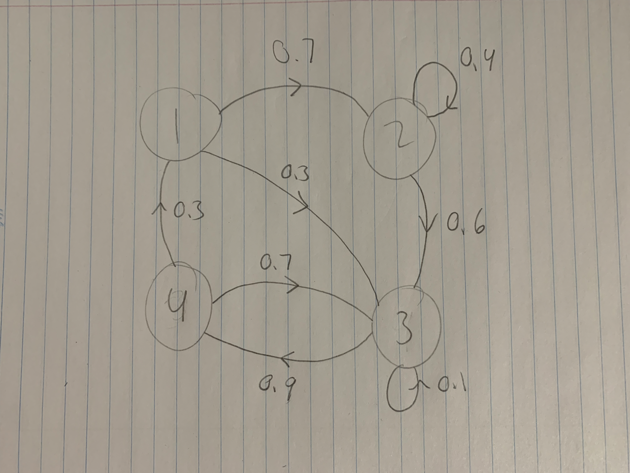
In this example, we can begin at any point and reach any other point. For example, from state 2, we can get to states 3, 4, 1, and state 2 itself. The same is true for states 1, 3, and 4. Thus, the Markov Chain is irreducible.
In an irreducible chain, all states have the same period. In the example above, this common period is 1. To see this, at least for states 1 and 2, we can observe that state 2 has a loop to itself, and so its period is 1. For state 1, we can consider the path \(1\rightarrow2\rightarrow3\rightarrow4\rightarrow1\), which has length 4 (there are 4 transitions along this path), and the path \(1\rightarrow2\rightarrow2\rightarrow3\rightarrow4\rightarrow1\), which has length 5. The period of a state is the greatest common divisor of the lengths of all paths leading from that state back to itself, but in this case, we can already observe that \(gcd(4,5)=1\), and so state 1 has period 1 as well. Similar arguments can be used to show that states 3 and 4 also have period 1.
An irreducible chain in which all states have period 1 is called aperiodic. Aperiodicity is another condition required to guarantee that the states of a Markov Chain will have a stationary distribution.
Steaty-State Convergence Theorem
Theorem: If a Markov Chain is irreducible, positive recurrent, and aperiodic, then the steady-state probabilites of the state space of the chain converge to a stationary distribution \(\pi\). Moreover, this stationary distribution \(\pi\) does not depend on the initial state of the Markov Chain [this result is essentially copied from reference 1, page 58].
So, under the conditions of being irreducible, positive recurrent, and aperiodic, we are guaranteed to have a Markov Chain whose steady-state probabilities converge in the long run to some distribution \(\pi\), called the stationary distribution of the chain.
A simple example of this would be the following. Consider a Markov Chain with a state space \(\{1,\:2\}\), where the transition matrix is given by
\[ \mathbb{P}= \begin{bmatrix} 0.5 & 0.5 \\ 0.5 & 0.5 \end{bmatrix}. \]
This Markov Chain is irreducible, positive recurrent, and aperiodic, and so the steady-state probabilities converge to a certain stationary distribution \(\pi\). In this case, either state is equally likely to remain at itself for the next time step or to move to the other state. Thus, we would expect that the stationary distribution would be \(\pi=\{\pi_1=0.5,\:\pi_2=0.5\}\). The interpretation of this stationary distribution is that we would expect the chain to be at state 1 fifty percent of the time and for the chain to be at state 2 for fifty percent of the time.
Markov Chain Monte Carlo
We are now ready to present Markov Chain Monte Carlo integration. Although this technique requires infinite state space Markov Chains in most cases, the ideas that we have explored in the previous section will carry through and help with the intuition behind certain aspects of MCMC.
We have previously seen how to solve a broad class of integrals using Monte Carlo integration techniques. Recall that in that setting, the goal was to frame an integral into one of the form
\[ \int_a^bg(x)f(x)dx, \]
where \(a\) and \(b\) are real values (possibly infinite) and \(f\) is a density function. By doing this, approximating such an integral then boils down to approximating \(E[g(X)]\). We can do this using the estimator
\[ \frac{1}{m}\sum_{i=1}^mg(X_i), \]
where the \(X_i\) form a random sample from the distribution \(f\). The issue that sometimes arises with this in practice, however, is that it can be quite difficult to generate independent samples from \(f\). Where Markov Chain Monte Carlo comes into play is that even with dependent samples, the integral can be approximated as long as the samples are generated in such a way that their joint density is approximately the same as the joint density of a random sample. Under certain circumstances, Markov Chain Monte Carlo does exactly this.
The idea is that, if \(\{X_0,\:X_1,\:X_2,...\}\) is a realization of an irreducible, positive recurrent, aperiodic Markov Chain with stationary distribution \(\pi\), then
\[ \overline{g(X)}_m=\frac{1}{m}\sum_{t=0}^mg(X_t) \]
converges with probability 1 to \(E[\,g(X)\,]\) as \(m\rightarrow\infty\), where \(X\) has the stationary distribution \(\pi\) and the expectation is taken with respect to \(\pi\) (provided the expectation exists) [this result is copied from reference 1, page 299]. The problem is then reduced to creating such a Markov Chain whose stationary distribution \(\pi\) is in fact the density \(f\) we were trying to sample from in the first place.
We will discuss one particular algorithm of MCMC called the Metropolis-Hastings Algorithm.
Metropolis-Hastings Algorithm
In any Metropolis-Hastings sampling algorithm (there are many such algorithms, each of which may be catered to a specific application. They essentially all follow the same general idea), the key idea is to specify how to select a point \(X_{t+1}\) in a Markov Chain when given a point \(X_t\) in the chain, and to make sure that the sample comes from the distribution \(f\) of interest for the integration problem.
In this type of sampling algorithm, a candidate point \(Y\) is generated from a proposal distribution \(g(\,\cdot\,|\,X_t\,)\). Then, a certain condition is checked to determine whether to accept or reject the candidate point \(Y\). If the point \(Y\) is accepted, then we set \(X_{t+1}=Y\); if \(Y\) is rejected, then \(X_{t+1}=X_t\). We then repeat the process.
The algorithm is similar to an acceptance-rejection one. We have seen that acceptance-rejection methods can be slow to implement, especially if we are rejecting most of the generated sample points. However, the power of Markov Chains in this context is that each next generated sample point is dependent on the previous sample point. Thus, if our previous sample point was chosen from an unlikely portion of the target distribution, then by the nature of the algorithm and Markov Chains, the procedure will essentially ‘correct’ for that and choose the next sample point in a more important portion of the distribution. This makes it so that rejecting sample points becomes less likely, and in any case, even if the sample point is rejected, we simply choose the next sample point to be the same sample point as before, and so we aren’t really losing observations.
The proposal distribution \(g(\,\cdot\,|\,X_t\,)\), can depend on the previous state of the Markov Chain. For instance, if we chose the proposal distribution to be \(g(\,\cdot\,|\,X_t\,)\sim\gamma(\,\alpha=3,\:\beta=X_t\,)\), then the \(\beta\) parameter of the proposal distribution would change whenever the \(X_t\) changes.
This process of generating sample points would be repeated until the chain has been running for a long enough time to have approximately reached its stationary distribution. The sample points that have been generated up to this point would not be used, and the chain would be run for a longer time to begin collecting sample points from that point onwards. This ensures that all sample points considered are in fact sampled from the required distribution.
When choosing an appropriate proposal distribution, one must keep in mind that the resulting Markov Chain must be irreducible, positive recurrent, and aperiodic in order to be guaranteed to have a stationary distribution. Usually, choosing a proposal distribution that is defined on the same domain as the target distribution will make it so that the stationary distribution of the resulting Markov Chain will have the same distribution as \(f\).
The details of the algorithm for the Metropolis-Hastings Sampler are as follows [as given in reference 1, page 300]. To generate the Markov Chain \(\{X_0,\:X_1,\:X_2,...\}\):
Choose a proposal distribution \(g(\,\cdot\,|\,X_t\,)\) (subject to the conditions given above).
Generate \(X_0\) from a distribution \(g\).
Repeat (until the chain has converged to its stationary distribution or at least approximately so; then start picking your samples points from here on out):
Generate \(Y\) from \(g(\,\cdot\,|\,X_t\,)\).
Generate \(U\) from \(Uniform(0,1)\).
If \(U\leq\frac{f(Y)g(X_t|Y)}{f(X_t)g(Y|X_t)}\), then accept \(Y\) and set \(X_{t+1}=Y\); otherwise, set \(X_{t+1}=X_t\).
Increment \(t\).
In the third part of step 3, the candidate point \(Y\) is accepted with probability
\[ \alpha(X_t,Y)=min\left(1,\frac{f(Y)g(X_t|Y)}{f(X_t)g(Y|X_t)}\right), \]
which means that the density \(f\) need only be known up to a constant (note that knowing how to plug a value into \(f\) and being able to randomly sample from \(f\) are two very different things, the first being much easier than the last in many cases).
It can be shown (the details are more involved than what can be shown in this document) that the stationary distribution of the Markov Chain is indeed the target distribution \(f\).
Applications
Markov Chain Monte Carlo integration is ubiquitous in the many branches of science and statistics. It has become indispensable in computational disciplines; areas such as computational physics, computational biology, and computational linguistics routinely use such methods in high-dimensional problems that would be intractable without them. Many simulations of physical systems rely on MCMC, from fluid flow to astrophysical systems. In statistics, Bayesian Inference is heavily reliant on MCMC to integrate various integrals that come up in the subject.
Overall, MCMC is an extension to regular Monte Carlo Methods that expands the horizon for the problems that Monte Carlo methods can tackle. Without it, many advancements in modeling and approximating mathematically intractable integrals would have been much more arduous.
References
Note that much of this work was modeled off of the lecture videos from [4], [5], and [6], and from the textbook from [1].
[1] Rizzo, M. L. Statistical Computing with R. 2nd edition. Taylor and Francis Group, 2019.
[2] Wikipedia. (2024). Stochastic Process. https://en.wikipedia.org/wiki/Stochastic_process
[3] Wikipedia. (2024). Markov chain Monte Carlo. https://en.wikipedia.org/wiki/Markov_chain_Monte_Carlo
[4] MIT 6.041: Probabilistic Systems Analysis and Applied Probability. Lecture 16: Markov Chains I. [Video] MITOpenCourseWare; 2010. https://ocw.mit.edu/courses/6-041-probabilistic-systems-analysis-and-applied-probability-fall-2010/resources/lecture-16-markov-chains-i/
[5] MIT 6.041: Probabilistic Systems Analysis and Applied Probability. Lecture 17: Markov Chains II. [Video] MITOpenCourseWare; 2010. https://ocw.mit.edu/courses/6-041-probabilistic-systems-analysis-and-applied-probability-fall-2010/resources/lecture-17-markov-chains-ii/
[6] MIT 6.041: Probabilistic Systems Analysis and Applied Probability. Lecture 18: Markov Chains III. [Video] MITOpenCourseWare; 2010. https://ocw.mit.edu/courses/6-041-probabilistic-systems-analysis-and-applied-probability-fall-2010/resources/lecture-18-markov-chains-iii/
[7] Statistics 110: Probability. Lecture 31: Markov Chains. [Video] Harvard University; 2013. https://www.youtube.com/watch?v=8AJPs3gvNlY
[8] Dr. Trefor Bazett. Intro to Markov Chains & Transition Diagrams. [Video] Discrete Math (Full Course: Sets, Logic, Proofs, Probability, Graph Theory, etc). https://www.youtube.com/watch?v=rHdX3ANxofs&list=PLHXZ9OQGMqxersk8fUxiUMSIx0DBqsKZS&index=78
[9] Dr. Trefor Bazett. Markov Chains & Transition Matrices. [Video] Discrete Math (Full Course: Sets, Logic, Proofs, Probability, Graph Theory, etc). https://www.youtube.com/watch?v=1GKtfgwf3ig&list=PLHXZ9OQGMqxersk8fUxiUMSIx0DBqsKZS&index=80
[10] ritvikmath. Markov Chain Monte Carlo (MCMC): Data Science Concepts. Data Science Concepts. https://www.youtube.com/watch?v=yApmR-c_hKU
[11] ritvikmath. Metropolis - Hastings: Data Science Concepts. Data Science Concepts. https://www.youtube.com/watch?v=yCv2N7wGDCw