# Calculate R-squared for the saturated model
risk_function <- function(dataframe) {
  # Requires sufficient n for the interaction terms
  if(nrow(dataframe) < 12) return(0)
  m <- lm(y ~ x * w * z, data = dataframe)
  summary(m)$r.squared
}

variance_function <- function(existing_df, newdat) {
    # This function measures the uncertainty associated with a new point
    # Right now I am using the standard error of prediction from the
    # regression model, as this gives a sense as to how uncertain a given
    # point is.
    # I suspect in CDOC, this is actually tied more directly to the
    # objective function; but this may work for a simulated proxy.

    predict(lm(y ~ x*w*z, data = existing_df), newdata = newdat, se.fit = TRUE)$se.fit

}

# The generative outcome function (Standard Case)
generate_outcome_default <- function(x, w, z) {
  5 + 5*x + 2*w + 1*z + 5*x*w + rnorm(length(x), 0, 10)
}

# Simulation Runner: Iteratively recruits based on R^2
run_simulation <- function(n_steps = 20,
                           outcome_func = generate_outcome_default,
                           seed_size = 12,
                           curiosity_lambda = 0.85,
                           x_range = 1:10,
                           w_range = 0:1,
                           z_range = -1:1,
                           random = FALSE,
                           iterative = TRUE) {

  # Search Space
  all_opts <- expand.grid(x = x_range, w = w_range, z = z_range)

  # Initial Seed
  seed_indices <- sample(1:nrow(all_opts), seed_size, replace = TRUE)
  current_df <- all_opts[seed_indices, ]
  current_df$y <- outcome_func(current_df$x, current_df$w, current_df$z)

  # Oracle Truth
  all_opts$y_truth <- outcome_func(all_opts$x, all_opts$w, all_opts$z)

    if(iterative) {
        history <- data.frame(step = integer(), r_squared = double())
        selections <- c()

        for(i in 1:n_steps) {

            if(random) {
                best_idx <- sample(1:nrow(all_opts), 1)
            } else {
                rewards <- numeric(nrow(all_opts))

                if(runif(1) <= curiosity_lambda) {
                    # Exploit
                    for(j in 1:nrow(all_opts)) {
                        candidate <- all_opts[j, ]
                        candidate$y <- candidate$y_truth
                        temp_df <- rbind(current_df, candidate[, c("x","w","z","y")])
                        rewards[j] <- risk_function(temp_df)
                    }

                } else {
                    # Explore
                    for(j in 1:nrow(all_opts)) {
                        candidate <- all_opts[j, ]
                        candidate$y <- candidate$y_truth
                        rewards[j] <- variance_function(current_df, candidate)
                    }

                }

                best_idx <- which.max(rewards)
            }

            best_candidate <- all_opts[best_idx, ]
            best_candidate$y <- best_candidate$y_truth

            current_df <- rbind(current_df, best_candidate[, c("x","w","z","y")])
            selections <- rbind(selections, best_candidate %>% mutate(step = i))
            history <- rbind(history, data.frame(step = i, r_squared = risk_function(current_df)))

            # Regenerate 'truth' for the selected individual
            all_opts$y[best_idx] <- outcome_func(all_opts$x[best_idx], all_opts$w[best_idx], all_opts$z[best_idx])
        }
    } else {
        # Only use random selection if non-iterative.
        selections <- sample(1:nrow(all_opts), n_steps, replace = TRUE)
        all_vars <- all_opts[selections, ]
        all_vars$y <- outcome_func(all_vars$x, all_vars$w, all_vars$z)
        current_df <- rbind(current_df, all_vars[, c("x","w","z","y")])
        history <- data.frame(step = n_steps, r_squared = risk_function(current_df))
    }
  list(selections = selections, history = history, final_df = current_df)
}

sim1 <- run_simulation(n_steps = 100, curiosity_lambda = 0.5, seed_size=20, x_range = 0:10)
sim2 <- run_simulation(n_steps = 100, random=TRUE, seed_size=20, x_range = 0:10)Discussion of \(R^2\) as a Cost Function for Curiosity-Driven Optimal Control
Executive Summary
There are some pieces that are unclear to me regarding how the algorithm will be operationalized in practice (e.g., relating to what probing means exactly and what the unit we should be probing is). Some of this confusion, I think, stems from the fact that we are using CDOC as a metaalgorithm of sorts, which may in turn necessitate a deeper specification of the underlying algorithm or process. Layered on top of this, there are some possible, mathematical issues regarding \(R^2\), or other measures of model fit, that I think may cause problems; though, curiosity may help to remedy this to some extent. The potential concerning behaviour is evident in simulations – both artbirary, and in some that are motivated via heart attack problems. I also spend some time exploring where we may go next.
The questions/overarching comments are likely the most important to directly address; further, some future possibilities are provided afterwards. I recognize there is a lot here, but I do not think that most of it needs to be addressed in detail (it was largely “for me” to explore the problem).
Some Questions/Overarching Comments
I believe that I require some additional clarity on what it might mean to “probe” a particular variate. In our setup, the algorithm would be selecting which individual should be selected next. As such, in a sense, it is capable of probing all factors at once. Is this correct?
- If this is correct, then should we instead be thinking about probing as based on the individual (as in, what set of factors) rather than the trait?
- If this is not correct, what does it look like to “probe” a trait, in practice.
I think that, for me, it seems as though the problem may need to be defined with additional depth. In a sense, I am wondering: what is our ultimate goal in this setting? My initial instinct is that the vision is (vaguely):
to promote equitable research by ensuring diversity of participants along the axes that are of material importance.
(I may be slightly off here, but I suspect this is at least in the same ballpark as others). The difficulty I have with this vision, is that I am not sure it is actionable (at this moment, without further clarity).
- In the DOID example, the actions taken have the ultimate goal of getting you to work – the quality of this depends primarily on the speed. As such, the actions that need to be taken relate to driving a car, and we will know it has been successful if it navigates the car to the destination quickly.
- To move this into our setting, the actions taken are proposed individuals to recruit to the study. How will we know that it has been successful? I think that this is simply a parallel question to “what should the cost function be”; however, phrased like this, I have some different considerations. Namely, the curiosity framework here is instrumental to some other goal that depends on the context: what is that goal?
- Is the scientific goal ultimately to do some type of “model discovery”?
- Is the scientific goal ultimately to recommend the best treatments?
- Is the scientific goal ultimately to be able to predict outcomes effectively?
- I would like to be able to fill in the blank: “If CDOC works well for this scenario, we would see ___.”
- Part of what I feel that I am getting at here is that, for us, CDOC is being used as a metaalgorithm. There is the scientific process that is (hypothetically) happening underneath, and we are trying to use CDOC as an input (or supplement) to that. As such, there may need to be some degree of specification of what the underlying component is, in order to ensure that CDOC is effective (or that we can define what it means to be effective). I am not sure that we can remain entirely agnostic to what the goal of the analysis is for the hypothetical experiment that we are recruiting for. Some thoughts:
- May we want to consider either the power calculation or p-values? If the goal is hypothesis testing, and discovering true interactions, this may be a method to proceed?
- May we want to consider model selection? If the contention is that we want to better understand how different factors impact outcomes, then this likely can only be accomplished by trying to find more descriptive models.
- May we want to consider some form of a validation set, and the model performance there?1
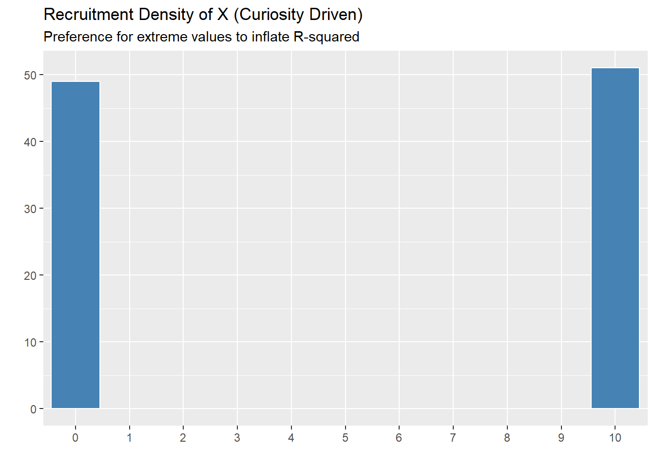
With \(R^2\) directly, or in fact many similar measures, I have some concerns about the possibility of it be exploited by the algorithm in a few different ways.
- Reward-hacking is possible by the algorithm picking two different points back and forth (supposing we are using a linear regression). This behaviour arises in the simulations below.
- In order to use our traditional interpretations of \(R^2\), there is a sense in which \(R^2\) should be independent of the data. It has a theoretical value to which it converges in the limit, supposing that data are actually selected from everywhere (representatively across the population).
- It is possible to remain above this theoretical value by artificially selecting data that fit more neatly. Instead of learning about the entire population, the model would be restricted to learning about the part of the population where the model fits nicely.
- This may cause concerns as an optimization metric (as \(n\) increases). More concerningly, however, is that it feels like it is explicitly counter to our goals. Perhaps some of this is alleviated by the curiosity component, though, my understanding is that curiosity is only leveraged when the thought is that, by learning more about a particular part of the space, the long-term objective will be better off. In practice, with \(R^2\), by learning more thoroughly about the entire space, the long-term objective may well be worse off.
Do we need to have some explicit measure of diversity captured here? Again, this feels like it may be difficult to do, and perhaps is counter to the point (or, at least, if our goal is maximize diversity, it seems likely that this would not be leveraging very well the curiosity driven components of it). This is where I perhaps harken back to point (2) and wonder, in practice, what is the goal of the recruitment for the individuals.
Simulations and Research Notes
Note: the following are essentially research “lab notes”; they follow my natural thought process to work through an assessment of \(R^2\) as a possible metric, edited slightly to make them more useful for others. They are somewhat verbose, as they map everything along the process.
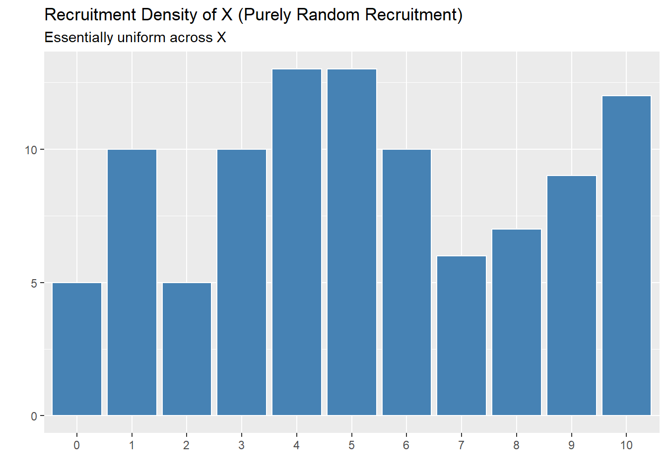
To demonstrate the concerns with \(R^2\) as a metric, lets consider a simulation setup. We can compare (in a simplified environment) random selection, a greedy algorithm, and a proxy for the curiousity-driven algorithm.
Original Simulation
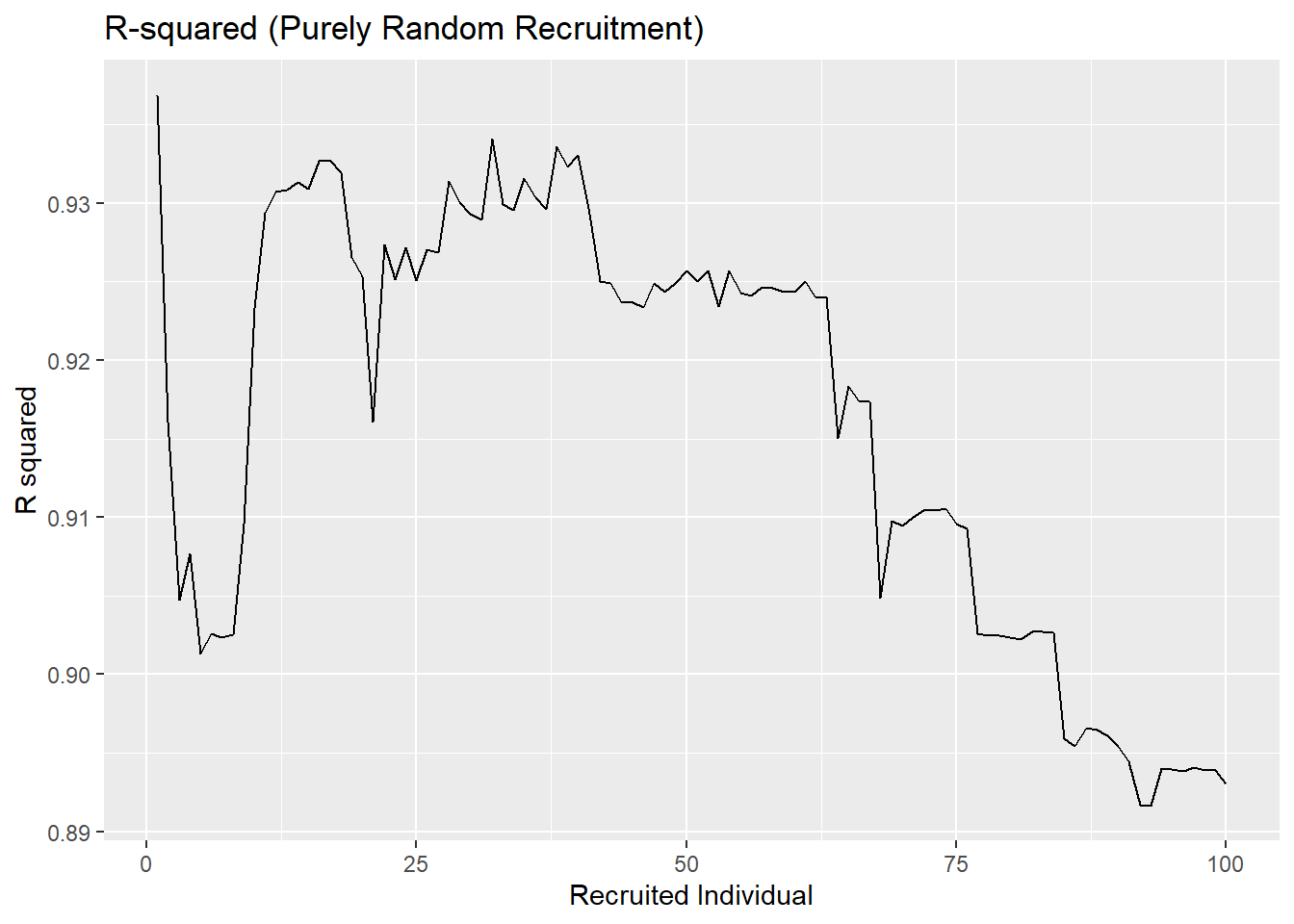
To implement the curiosity-driven proxy: start from the greedy algorithm, and 50% of the time, pick the individual who has the highest predictive uncertainty. The other 50% of, pick the individual that will maximize the \(R^2\). Note that the selection is based on a greedy Oracle algorithm (as in, it actually knows the \(R^2\) that will be found and searches every point). I recognize this is not a perfect encapsulation of “curiosity” here, however, even just looking at the oracle shows how \(R^2\) can be exploited. This is compared to a version of the algorithm that just uses completely random selection.
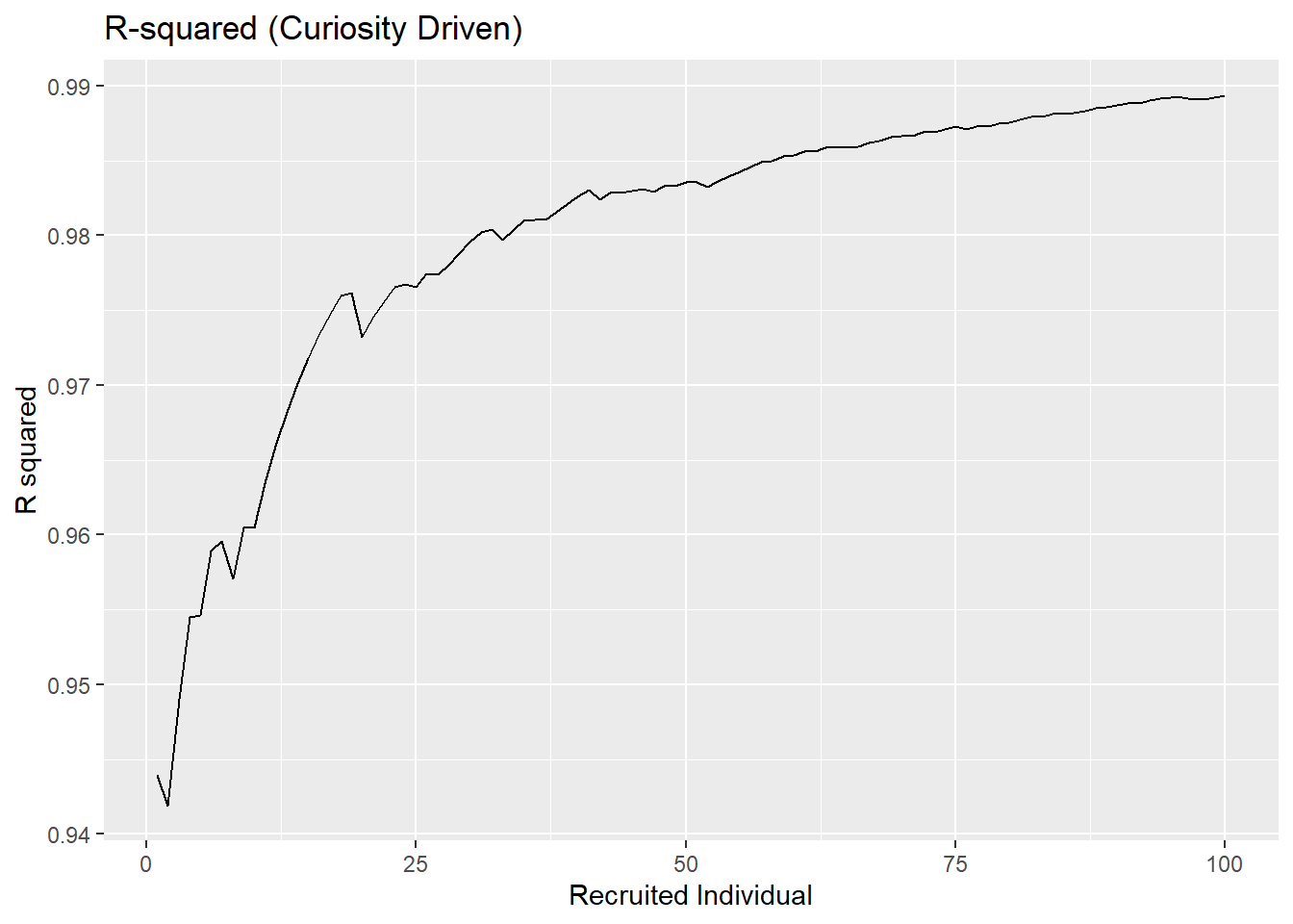
Note, that if 50-50 split is changed, the same patterns emerge.
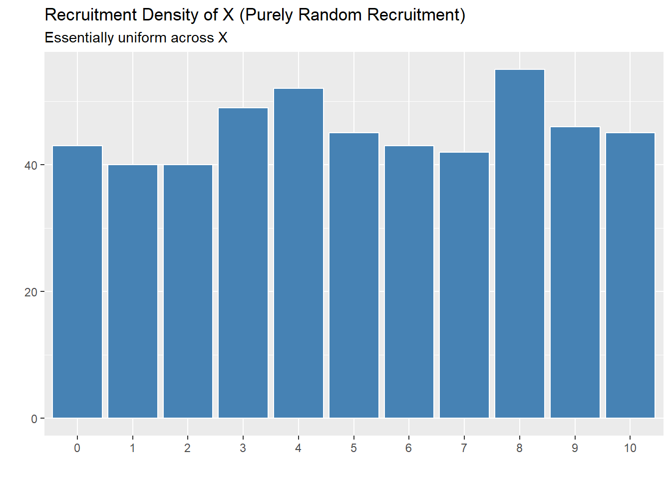
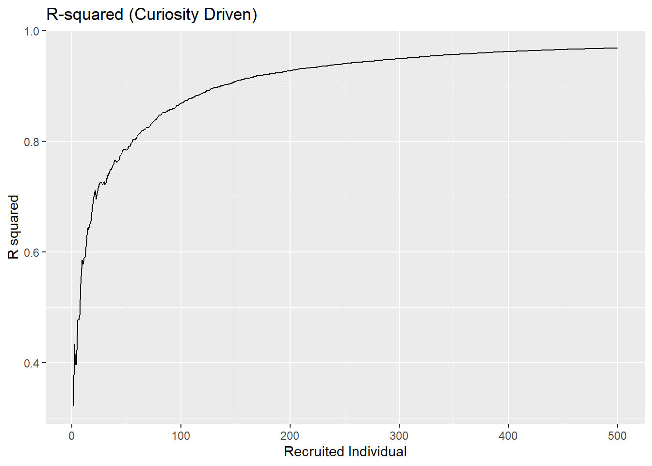
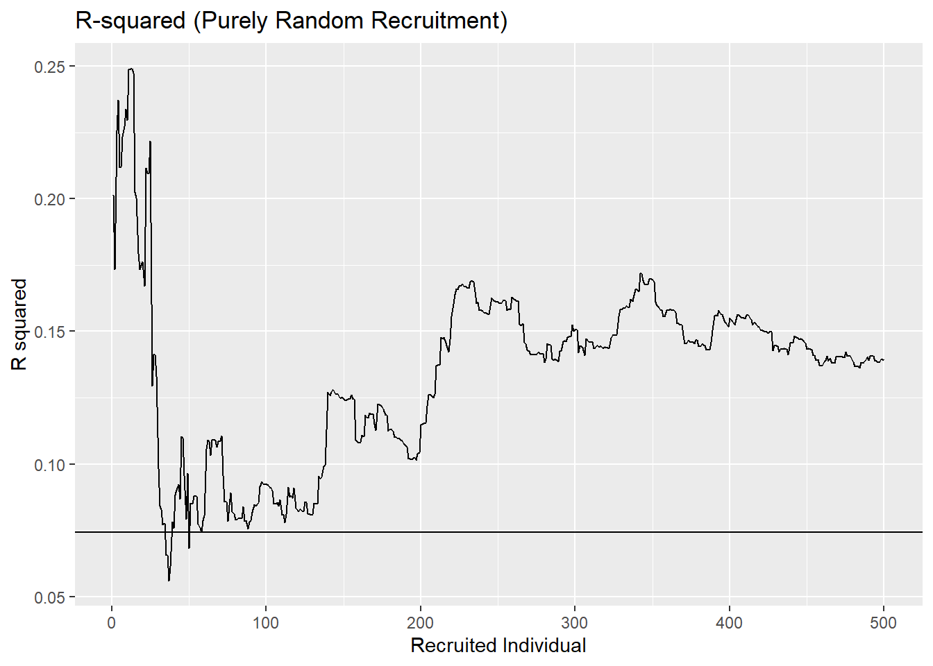
Simulation With a Worse Fit
If we imagine a situation with more noise in it (not changing anything else of note), then we can see an even starker difference between the \(R^2\) values with the curioisty approach and the random selection. We have the curiosity framework able to achieve an incredibly high \(R^2\) (around \(0.99\)) while the random approach tends much lower (around \(0.15\)) and would theoretically converge even lower than that (around \(0.05\)).
Code
# The generative outcome function (Standard Case)
generate_outcome_default <- function(x, w, z) {
  5 + 5*x + 2*w + 1*z + 5*x*w + rnorm(length(x), 0, 100)
}

sim3 <- run_simulation(n_steps = 500, curiosity_lambda = 0.5, seed_size=20, x_range = 0:10)
sim4 <- run_simulation(n_steps = 500, random=TRUE, seed_size=20, x_range = 0:10)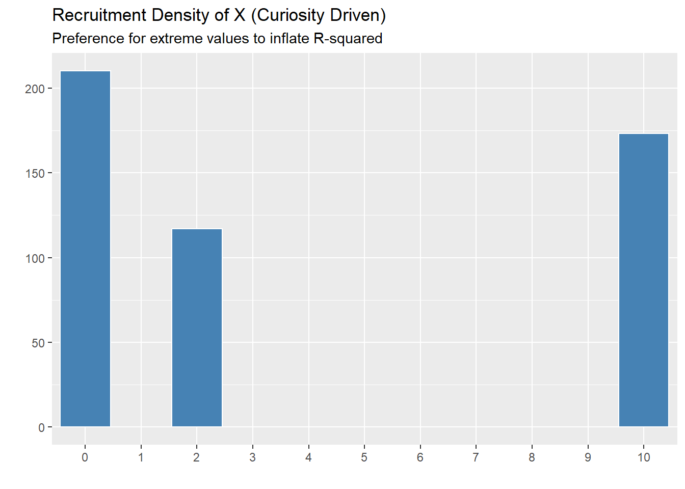
Connecting to MI Example
To help myself (and make matters concrete), I wanted to try to map this onto the MI example that Ande typically uses in the lead-in to the elevator pitch. Namely: if we had been doing recruitment for a study that was looking at troponin levels for the identification of an MI, would this have worked well?
The first issue that I foresee with this setup is that, given the chance, the algorithm will likely only pick those people who are very far from the cutoff barriers (that is, those people who have very low troponin or very high troponin levels). These people will be the easiest to predict, and so if we are using a metric that asks “how well does prediction proceed”, then this is likely what we will observe. In this example, there is also the possibility that both males and females have extreme values, and so some modest amount of diversity (both sex and troponin level) could be maintained. We would likely miss the middle values.
If we suppose that we had a restricted entrance into the study so that only people with elevated troponin measures were included (those near hypothetical barriers), then I think that the results might differ slightly. (This all assumes that there are not an abundance of individuals who are easy to select based on the aforementioned exploitable patterns.) If we imagine having seeded the study with males (as likely happened) and then considered the level that indicated a heart attack, we likely would have identified (with lots of noise) the usual level in males; say that this is around \(20\).2 If we suppose (unrealistic, but worthwhile for now) that the only thing that impacts the threshold to indicate a heart attack is sex, then any measure of model fit (such as \(R^2\) or related metrics) is going to remain high as long as those who we recruit are male.
Suppose that, based on curiosity, the algorithm proposes the recruitment of a female participant, who has a true level around \(15\). If we are using a single threshold to based our prediction off of to begin (as in, the underlying model did not start with prior knowledge that other factors would be important), the inclusion of the female subject will likely have the effect of lowering the \(R^2\). This, I think, will prompt the curiosity driven framework to learn that sampling in this part of the space is not a worthy pursuit (as it lowers the cost function), and it will turn back to other areas.3
If instead of a simple model, we had already included a term for sex in the model, then this leads to 3 interwoven thoughts:
- The \(R^2\) will likely be lower than it would have been, had a male patient been selected instead.
- The fact that the researchers already included sex in the model makes it suspect that (i) all the seed participants would be male, and (ii) calls into question precisely what benefit the CDOC approach would have here (if we know we need to recruit on sex, and it turns out that sex is the only thing that matters).
- Should we be considering model selection instead? If there is already a fixed model in place, then it is not immediately clear where there is space to gain using targeted recurimtent.4
Aside: In this example, in practice, I would think that the CDOC would not actually specify the troponin level for recruitment. I am not sure about the framing of this in the language of control problems, but troponin level here, while not the final outcome, is in a sense an intermediary outcome. If it seems worthwhile, I could add a simulation later that looks more effectively at selection, but for now, this can be a stnad-in for any similar situation where an actual predictive factor has these types of relationship.
Simulation of MI Setting
To attempt to simulate this setting, we take the following simulation setup. Every person has a set upperbound on their necessary troponin levels, observations beyond which indicate a heart attack. These levels are centered at the sex-specific values (\(20\) and \(15\) for males and females, respectively). Observations above this threshold occur if a heart attack happened, with almost perfect accuracy (\(99\%\) of time). The observed data for each individual is \(X\) (sex, \(1\) for female and \(0\) for male); \(W\) (troponin, a numerical value \(\geq 0\)); \(Y\) (heart attack indicator, \(1\) for yes and \(0\) for no).
Individuals are recruited to the study, and the model that is being fit is a logistic regression, that aims to predict the probability that an individual (with observed values \(x\) and \(w\)) had a heart attack. Specifically, we take \[\log\left(\frac{\pi}{1 - \pi}\right) = \beta_0 + \beta_1 X + \beta_2 W + \beta_3 XW.\] Here, \(\pi\) is the individual probability of a heart attack. Now, based on the values, we should find that \(\beta_0 \approx -20\beta_2\) and that \(\beta_0 + \beta_1 \approx -15(\beta_2 + \beta_3)\), or equivalently, that \(\beta_1 \approx 5\beta_2 - 15\beta_3\). The exact magnitude will depend on the overall proportion of individuals who were observed to have (or not have) heart attacks within each of the barriers.
In place of \(R^2\) (which is not really well-defined for logistic regression), I will report the mean squared error (or Brier Score). This is probably not the best, but in linear regression, MSE and \(R^2\) have a one-to-one mapping, and as such, this gets at the same idea.5
set.seed(31415)

# Set constants
MALE_LEVEL <- 20
FEMALE_LEVEL <- 15

# Assume a population size of 10,000 possible people exist
# In the population there is a ~50/50 split for male/female
POP_N <- 10000
population_df <- data.frame(
  sex = rbinom(POP_N, 1, 0.5),          # Sex indicator
  max_level = rnorm(POP_N, 0, 0.915),       # Noise on max troponin level
  heart_attack = rbinom(POP_N, 1, 0.1), # 10% of people have MIs
  observed_t = 0                        # Observed troponin; define later
)

# Generate the max levels and the observed troponin for the individuals;
# then swap the labels for heart attack for 1% of people
population_df$max_level <- population_df$max_level + MALE_LEVEL + population_df$sex * (FEMALE_LEVEL - MALE_LEVEL)
population_df$observed_t <- (1 - population_df$heart_attack) * runif(POP_N, 0, population_df$max_level) +
                            population_df$heart_attack * runif(POP_N, population_df$max_level, population_df$max_level + 3)

swap_idxs <- sample(1:POP_N, 0.01 * POP_N, FALSE)
population_df$heart_attack[swap_idxs] <- 1 - population_df$heart_attack[swap_idxs]
With the full population generated, we can then run the logistic regression model and consider the model output, if we had access to the full population.
Code
POP_model <- glm(heart_attack ~ sex * observed_t, data = population_df, family = "binomial")
POP_mse <- mean((population_df$heart_attack - predict(POP_model, type="response"))^2)

summary(POP_model)
Call:
glm(formula = heart_attack ~ sex * observed_t, family = "binomial",
    data = population_df)

Coefficients:
                Estimate Std. Error z value Pr(>|z|)
(Intercept)    -12.74113    0.51932 -24.534  < 2e-16 ***
sex             -1.08549    0.77019  -1.409    0.159
observed_t       0.62455    0.02667  23.420  < 2e-16 ***
sex:observed_t   0.26933    0.04682   5.752 8.82e-09 ***
---
Signif. codes:  0 '***' 0.001 '**' 0.01 '*' 0.05 '.' 0.1 ' ' 1

(Dispersion parameter for binomial family taken to be 1)

    Null deviance: 6833.6  on 9999  degrees of freedom
Residual deviance: 3125.5  on 9996  degrees of freedom
AIC: 3133.5

Number of Fisher Scoring iterations: 8
To check to ensure that the data generation is as we expect, we find that \(\frac{\beta_0}{\beta_2} \approx -20.4004\) and \(\frac{\beta_0 + \beta_1}{\beta_2 + \beta_3} \approx -15.468\), both as expected. We find the MSE at the population level to be \(0.0349\), which serves as a benchmark of performance.
Simulating Recruitment: Incorrect Model, Unrestricted
Next, we can attempt to simulate the recruitment process, comparing random recruitment to both a greedy search and a curiosity-driven recruitment. At first, we consider the incorrect model (that is, the one that ignores sex). We begin by seeding with \(20\) male participants, and then consider choosing the next best individual based on minimizing the MSE.6 The curiosity driven approach considers either taking the greedy search, or else selects at random.
Greedy Implementation
n_steps <- 50
seed_idxs <- sample(which(population_df$sex == 0), 20, FALSE)

# Pre-calculate the Model Matrix (Design Matrix)
X_full <- model.matrix(heart_attack ~ observed_t, data = population_df)
y_full <- population_df$heart_attack

# Keep track of indices
selectable_idx <- setdiff(1:POP_N, seed_idxs)
current_idxs <- seed_idxs
selected <- numeric(n_steps)
stepwise_MSE <- numeric(n_steps)
estimated_threshold <- numeric(n_steps)
HA_indicator <- numeric(n_steps)
troponin_vals <- numeric(n_steps)

for(ii in 1:n_steps) {
  cur_min_MSE <- Inf
  cur_select <- 0
  cur_thresh <- 0

  # Pre-extract the current X and y to avoid indexing inside the inner loop
  X_current <- X_full[current_idxs, , drop = FALSE]
  y_current <- y_full[current_idxs]

  for(jidx in selectable_idx) {
    # Combine current set with one candidate
    X_tmp <- rbind(X_current, X_full[jidx, ])
    y_tmp <- c(y_current, y_full[jidx])

    # Use speedglm.wfit for raw matrix input
    # This is significantly faster than the formula interface
    fit <- speedglm.wfit(y = y_tmp, X = X_tmp, family = binomial())

    # Fast prediction: 1 / (1 + exp(-X %*% beta))
    es_coefs <- coef(fit)
    eta <- X_tmp %*% es_coefs
    probs <- 1 / (1 + exp(-eta))

    tmp_mse <- mean((y_tmp - probs)^2)

    if(tmp_mse < cur_min_MSE) {
      cur_min_MSE <- tmp_mse
      cur_select <- jidx
      cur_thresh <- es_coefs[1]/es_coefs[2]
      cur_ha <- y_full[jidx]
      cur_trop <- population_df$observed_t[cur_select]
    }
  }

  selected[ii] <- cur_select
  stepwise_MSE[ii] <- cur_min_MSE
  estimated_threshold[ii] <- cur_thresh
  HA_indicator[ii] <- cur_ha
  troponin_vals[ii] <- cur_trop

  current_idxs <- c(current_idxs, cur_select)
  selectable_idx <- setdiff(selectable_idx, cur_select)
}
Curiosity-Driven Implementation
In the curiosity-driven framework here, I have played with the split. Instead of using the greedy algorithm 50% of the time, it uses it 85% of the time. Again, it appears as though the overarching patterns are not particularly sensitive to this choice. Further, instead of using the most uncertain, it falls back on completely random selection; when using the uncertainty measure directly here, the choices rarely deviated from the greedy selections.
Code
n_steps <- 50
lambda_c <- 0.85 # Proportion of the time to exploit
# Use the same seed_idxs as before

# Pre-calculate the Model Matrix (Design Matrix)
X_full <- model.matrix(heart_attack ~ observed_t, data = population_df)
y_full <- population_df$heart_attack

# Keep track of indices
selectable_idx <- setdiff(1:POP_N, seed_idxs)
current_idxs <- seed_idxs
selected_c <- numeric(n_steps)
stepwise_MSE_c <- numeric(n_steps)
estimated_threshold_c <- numeric(n_steps)
HA_indicator_c <- numeric(n_steps)
troponin_vals_c <- numeric(n_steps)
type_steps <- numeric(n_steps)

for(ii in 1:n_steps) {
  if(runif(1) <= lambda_c) {
    cur_min_MSE <- Inf
    cur_select <- 0
    cur_thresh <- 0
    cur_type <- 1

    # Pre-extract the current X and y to avoid indexing inside the inner loop
    X_current <- X_full[current_idxs, , drop = FALSE]
    y_current <- y_full[current_idxs]

    for(jidx in selectable_idx) {
      # Combine current set with one candidate
      X_tmp <- rbind(X_current, X_full[jidx, ])
      y_tmp <- c(y_current, y_full[jidx])

      # Use speedglm.wfit for raw matrix input
      # This is significantly faster than the formula interface
      fit <- speedglm.wfit(y = y_tmp, X = X_tmp, family = binomial())

      # Fast prediction: 1 / (1 + exp(-X %*% beta))
      es_coefs <- coef(fit)
      eta <- X_tmp %*% es_coefs
      probs <- 1 / (1 + exp(-eta))

      tmp_mse <- mean((y_tmp - probs)^2)

      if(tmp_mse < cur_min_MSE) {
        cur_min_MSE <- tmp_mse
        cur_select <- jidx
        cur_thresh <- es_coefs[1]/es_coefs[2]
        cur_HA <- y_full[jidx]
        cur_trop <- population_df$observed_t[cur_select]
      }
    }
  } else {
    cur_type <- 0
    cur_select <- sample(selectable_idx, 1)
    tmp_df <- population_df[c(current_idxs, cur_select), ]
    tmp_model <- glm(heart_attack ~ observed_t, data = tmp_df, family = "binomial")
    cur_min_MSE <- mean((tmp_df$heart_attack - predict(tmp_model, type="response"))^2)
    cur_thresh <- coef(tmp_model)[1]/coef(tmp_model)[2]
    cur_HA <- population_df$heart_attack[cur_select]
    cur_trop <- population_df$observed_t[cur_select]
  }

  selected_c[ii] <- cur_select
  stepwise_MSE_c[ii] <- cur_min_MSE
  estimated_threshold_c[ii] <- cur_thresh
  HA_indicator_c[ii] <- cur_HA
  troponin_vals_c[ii] <- cur_trop
  type_steps[ii] <- cur_type

  current_idxs <- c(current_idxs, cur_select)
  selectable_idx <- setdiff(selectable_idx, cur_select)
}
Random Implementation
Code
n_steps <- 50
lambda_c <- 0.85 # Proportion of the time to exploit
# Use the same seed_idxs as before

# Pre-calculate the Model Matrix (Design Matrix)
X_full <- model.matrix(heart_attack ~ observed_t, data = population_df)
y_full <- population_df$heart_attack

# Keep track of indices
selectable_idx <- setdiff(1:POP_N, seed_idxs)
current_idxs <- seed_idxs
selected_r <- numeric(n_steps)
stepwise_MSE_r <- numeric(n_steps)
estimated_threshold_r <- numeric(n_steps)
HA_indicator_r <- numeric(n_steps)
troponin_vals_r <- numeric(n_steps)

for(ii in 1:n_steps) {
  cur_select <- sample(selectable_idx, 1)
  tmp_df <- population_df[c(current_idxs, cur_select), ]
  tmp_model <- glm(heart_attack ~ observed_t, data = tmp_df, family = "binomial")
  cur_min_MSE <- mean((tmp_df$heart_attack - predict(tmp_model, type="response"))^2)

  selected_r[ii] <- cur_select
  stepwise_MSE_r[ii] <- cur_min_MSE
  estimated_threshold_r[ii] <- coef(tmp_model)[1]/coef(tmp_model)[2]
  HA_indicator_r[ii] <- population_df$heart_attack[cur_select]
  troponin_vals_r[ii] <- population_df$observed_t[cur_select]

  current_idxs <- c(current_idxs, cur_select)
  selectable_idx <- setdiff(selectable_idx, cur_select)
}
Results
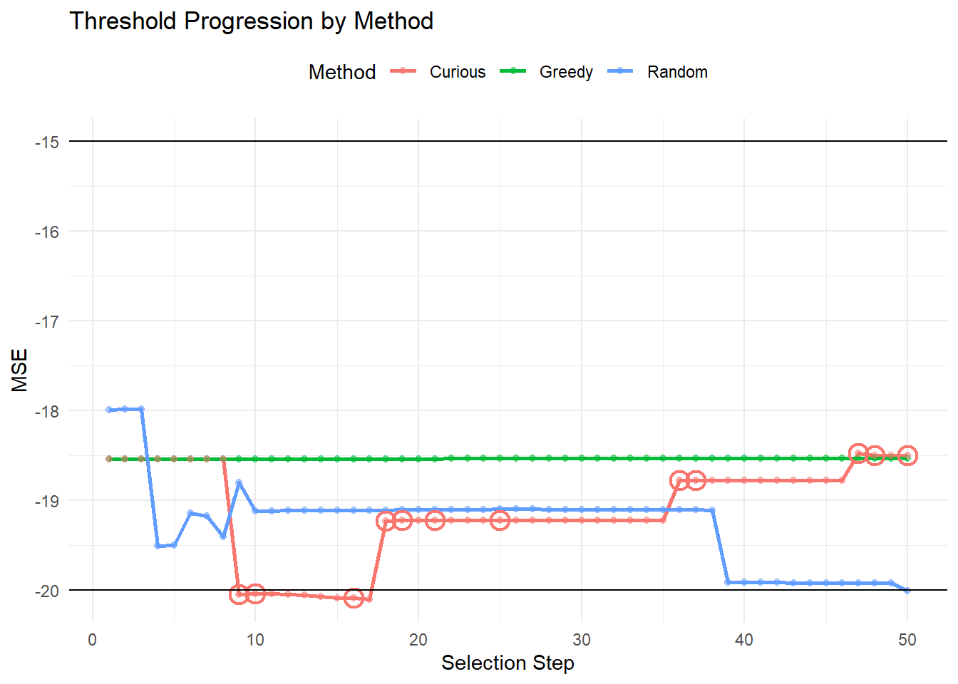
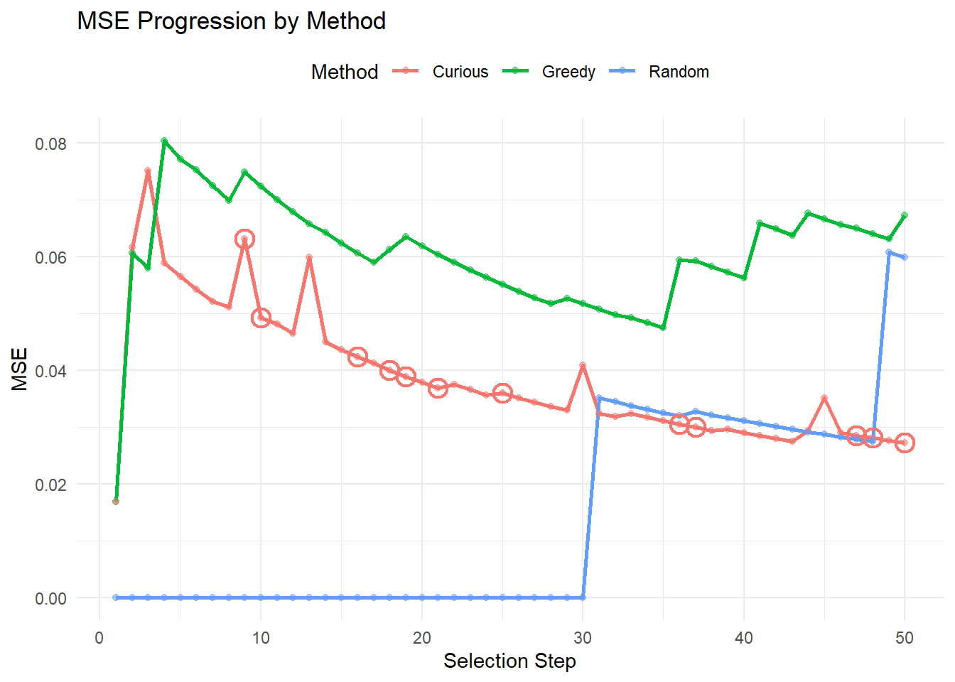
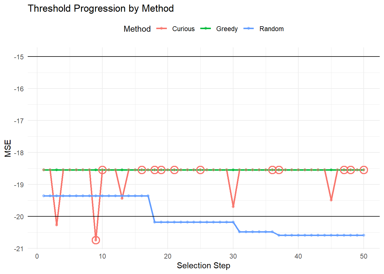
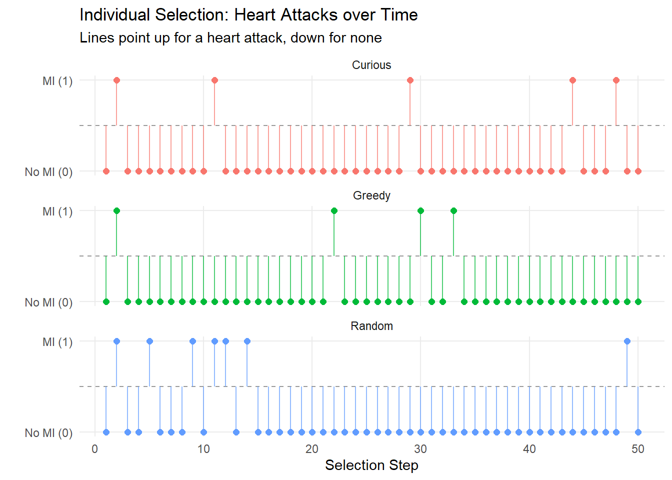
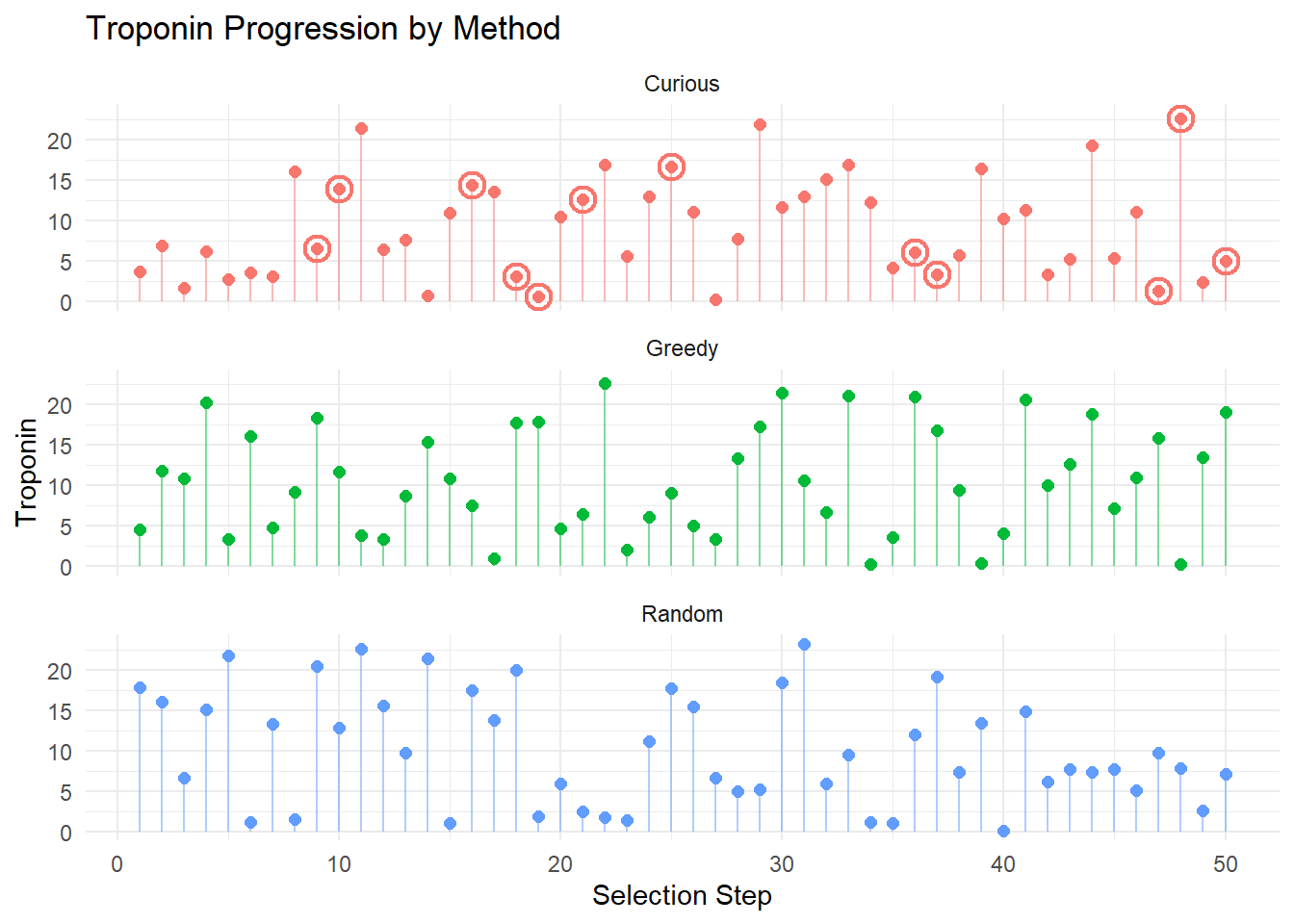
In the following we look at the results of the first run. These show the progression of the MSE over each recruited individual, the estimated treatment threshold, and then the sex/heart attack indicator status/troponin level for each selected individual. For the curiousity driven approach, points are circled when they corresponded to a random selection.
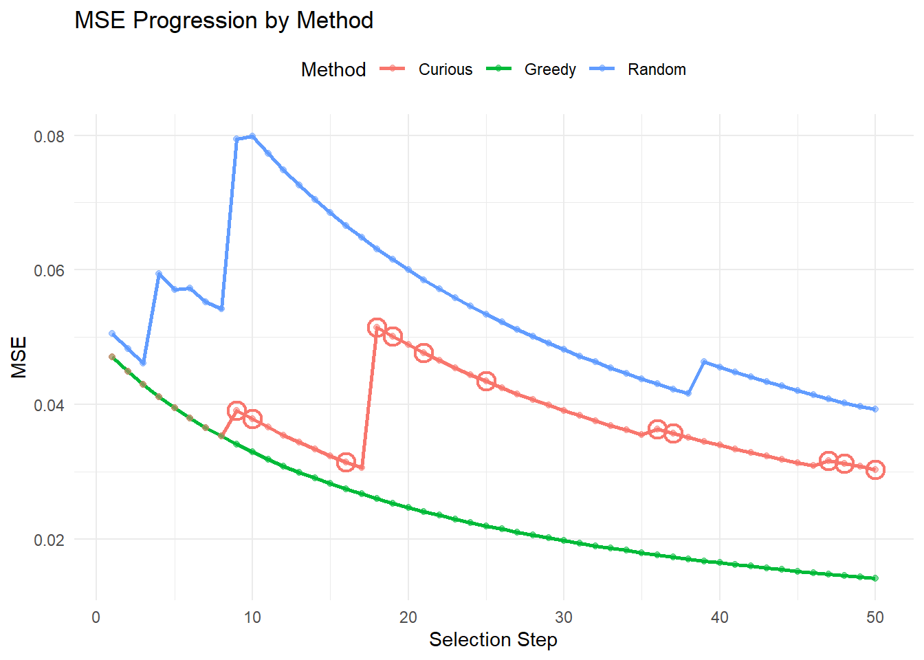
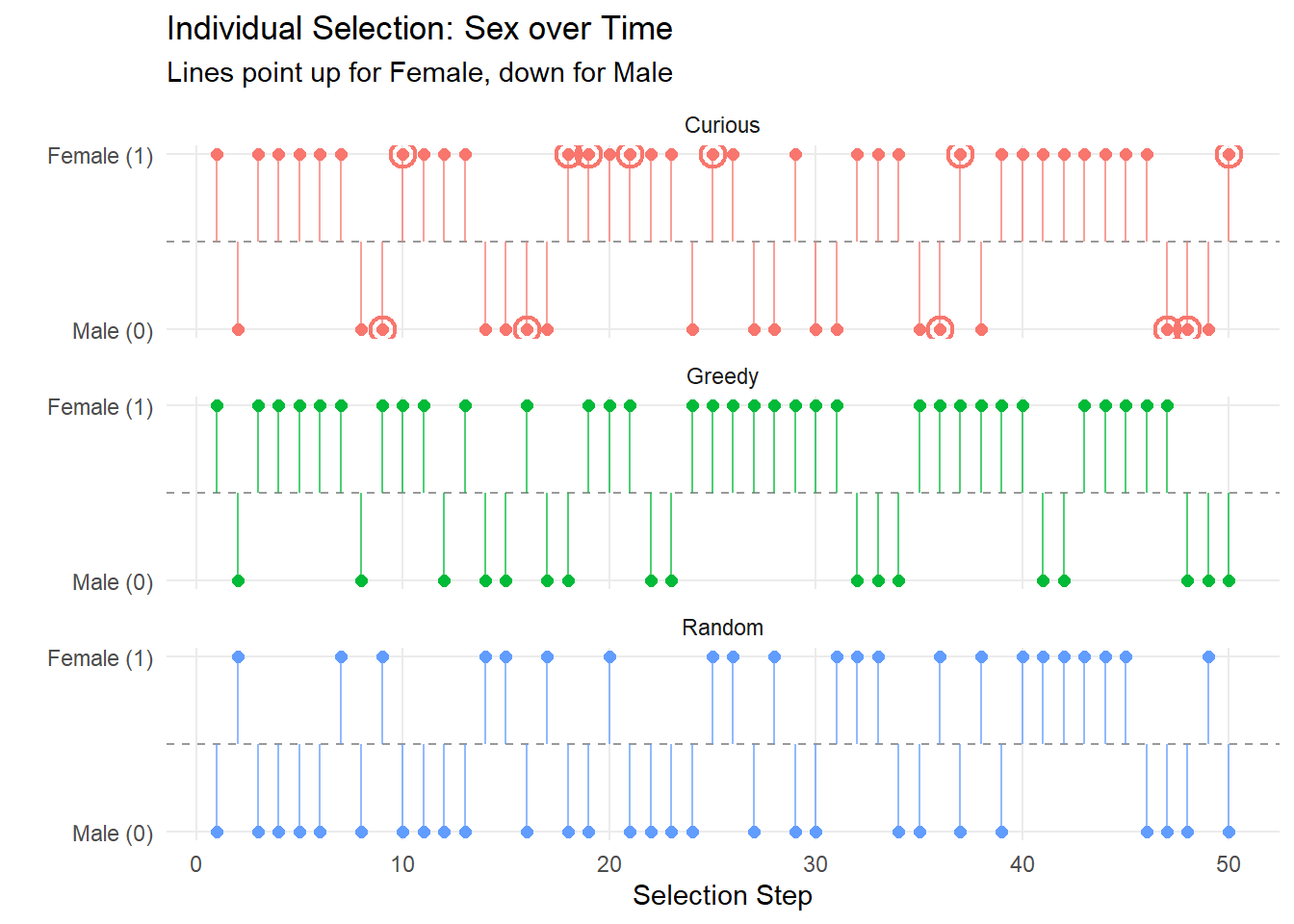
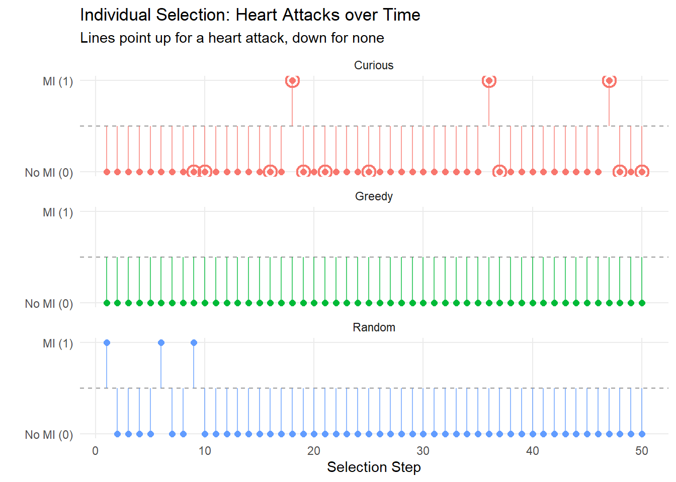
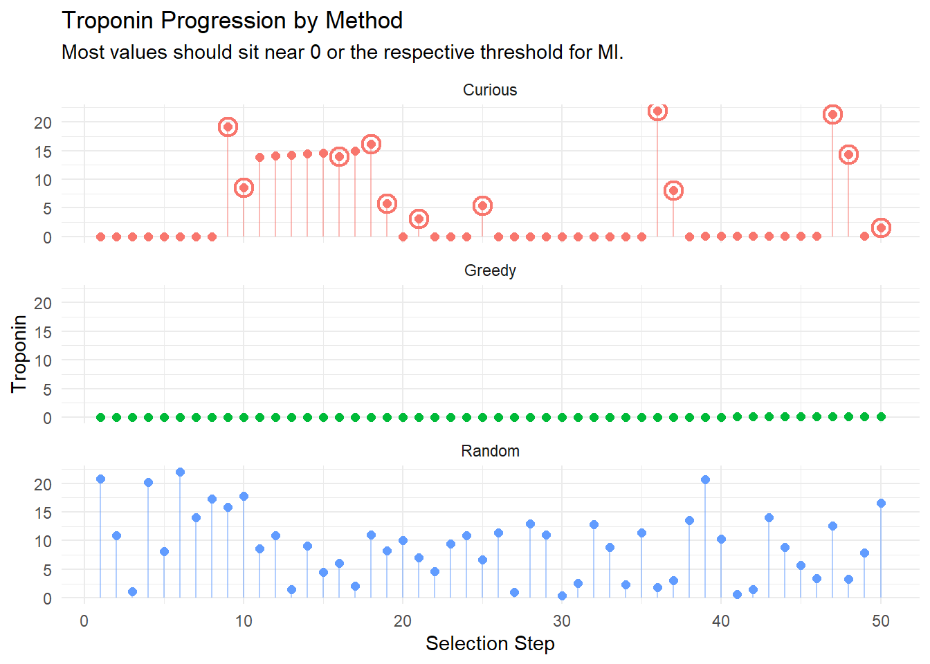
These results show what was expected: the greedy and curious algorithm lean very heavily on picking those participants who had never had heart attacks. Similarly, the greedy agent selected only those with (essentially) \(0\) for observed troponin; the curious model sat often around \(0\) as well, with ocassional spikes: note that the spikes tend to be when random selection was used (circled values).7
It is also worth checking what happens with the full population, if we use the incorrect model. To check to ensure that the data generation is as we expect, we find that \(\frac{\beta_0}{\beta_1} \approx -19.2637\). We find the MSE at the population level to be \(0.0577\), which serves as a benchmark of performance.
Note: The effects at work here at quite strong, in terms of selecting for extreme points (either low or high troponin, and either always MI present or never). These persist even when we limit the range of troponin values considered; I think largely because the effects in the simulated data are still too strong. Notably, in this particular setup, this does not necessarily lead to a sex-based bias, however, it has the same effect in principle. Because only extreme individuals are selected, the model is less likely to perform well on those who sit around the boundaries; this has a particular concern for females who have lower troponin levels when positive. Still, the selection bias based on sex is not obvious when troponin levels are available to be specified.
Sex-Based Selection
Consider if the algorithm can only make a decision based on sex, rather than selecting a specific troponin level as well. That is, the algorithm can only choose to recruit either a female or a male next, and then a random individual of that sex is recruited. To put this into practice, the greedy algorithm will consider the MSE that would result from recruiting each individual, and then select the sex that would lead to the lower MSE, with higher probability. The curiosity driven approach will either select the greedy choice, or else select totally at random. Random selection will proceed exactly as before. Note, because sex is being specifically targeted here in recruitment, we will also consider it in the model setup.
Greedy Implementation
Code
n_steps <- 50

# Seed with 15 males and 5 females; using sex we require some of each, but lets assume that the bias is towards males
# as is historically the case.
seed_idxs <- c(sample(which(population_df$sex == 0), 15, FALSE), sample(which(population_df$sex == 1), 5, FALSE))

# Pre-calculate the Model Matrix (Design Matrix)
X_full <- model.matrix(heart_attack ~ observed_t * sex, data = population_df)
X_full_simple <- model.matrix(heart_attack ~ observed_t, data = population_df)  # Fallback model
y_full <- population_df$heart_attack


# Keep track of indices
selectable_idx <- setdiff(1:POP_N, seed_idxs)
current_idxs <- seed_idxs
selected <- numeric(n_steps)
stepwise_MSE <- numeric(n_steps)
estimated_threshold <- numeric(n_steps)
HA_indicator <- numeric(n_steps)
troponin_vals <- numeric(n_steps)

for(ii in 1:n_steps) {
  # Compute MSE for ALL selectable individuals (not just the min)
  mse_list <- numeric(length(selectable_idx))
  thresh_list <- numeric(length(selectable_idx))
  ha_list <- numeric(length(selectable_idx))
  trop_list <- numeric(length(selectable_idx))

  # Pre-extract current X and y
  X_current <- X_full[current_idxs, , drop = FALSE]
  X_current_simple <- X_full_simple[current_idxs, , drop = FALSE]
  y_current <- y_full[current_idxs]

  for(k in seq_along(selectable_idx)) {
    jidx <- selectable_idx[k]
    # Combine current set with this candidate
    X_tmp <- rbind(X_current, X_full[jidx, ])
        X_tmp_simple <- rbind(X_current_simple, X_full_simple[jidx, ])
    y_tmp <- c(y_current, y_full[jidx])

    fit_result <- tryCatch({
        speedglm.wfit(y = y_tmp, X = X_tmp, family = binomial())
    }, error = function(e) {
        # Fallback to simplified model on any error (e.g., singularity)

        speedglm.wfit(y = y_tmp, X = X_tmp_simple, family = binomial())
    })

    es_coefs <- coef(fit)
    if(any(is.na(es_coefs))) {
    # If even simplified fails, set to Inf
    mse_list[k] <- Inf
    thresh_list[k] <- NA
  } else {
    # Check if we used the full model or simplified (based on matrix dimensions)
    if(ncol(X_tmp) == length(es_coefs)) {
      # Full model succeeded
      eta <- X_tmp %*% es_coefs
      thresh_list[k] <- es_coefs[1] / es_coefs[2]
    } else {
      # Fallback to simplified
      eta <- X_tmp_simple %*% es_coefs
      thresh_list[k] <- es_coefs[1] / es_coefs[2]  # Threshold from simplified model
    }
    probs <- 1 / (1 + exp(-eta))
    mse_list[k] <- mean((y_tmp - probs)^2)
  }

    ha_list[k] <- y_full[jidx]
    trop_list[k] <- population_df$observed_t[jidx]
  }

  # Group MSEs by sex
  sex_selectable <- population_df$sex[selectable_idx]
  mse_male <- mse_list[sex_selectable == 0]  # Males
  mse_female <- mse_list[sex_selectable == 1]  # Females

  # Compute P(X < Y): Probability a random male has lower MSE than a random female
  if(length(mse_male) == 0) {
    prob_male_better <- 0  # No males, select female
  } else if(length(mse_female) == 0) {
    prob_male_better <- 1  # No females, select male
  } else {
    # Sort female MSEs for binary search
    mse_female_sorted <- sort(mse_female)
    # For each male MSE, count females with lower MSE
    counts <- sapply(mse_male, function(m) {
      # findInterval gives the index where m would be inserted (0-based)
      idx <- findInterval(m, mse_female_sorted, rightmost.closed = FALSE)
      idx  # Number of females with MSE < m
    })
    prob_male_better <- mean(counts) / length(mse_female)  # Average proportion
  }

  # Decide sex based on probability
  if(prob_male_better > 0.5) {
    chosen_sex <- 0  # Male
  } else if(prob_male_better < 0.5) {
    chosen_sex <- 1  # Female
  } else {
    chosen_sex <- sample(c(0, 1), 1)  # Indifferent, random
  }

  # Select random individual from chosen sex
  sex_candidates <- selectable_idx[sex_selectable == chosen_sex]
  if(length(sex_candidates) == 0) {
    # Fallback if no candidates (shouldn't happen, but safety)
    cur_select <- sample(selectable_idx, 1)
  } else {
    cur_select <- sample(sex_candidates, 1)
  }

  # Record values for the selected individual
  idx_in_list <- which(selectable_idx == cur_select)
  selected[ii] <- cur_select
  stepwise_MSE[ii] <- mse_list[idx_in_list]
  estimated_threshold[ii] <- thresh_list[idx_in_list]
  HA_indicator[ii] <- ha_list[idx_in_list]
  troponin_vals[ii] <- trop_list[idx_in_list]

  # Update indices
  current_idxs <- c(current_idxs, cur_select)
  selectable_idx <- setdiff(selectable_idx, cur_select)
}
Curiosity-Driven Implementation
Code
n_steps <- 50
lambda_c <- 0.85 # Proportion of the time to exploit
# Use the same seed_idxs as before

# Pre-calculate the Model Matrix (Design Matrix)
X_full <- model.matrix(heart_attack ~ observed_t * sex, data = population_df)
y_full <- population_df$heart_attack

# Keep track of indices
selectable_idx <- setdiff(1:POP_N, seed_idxs)
current_idxs <- seed_idxs
selected_c <- numeric(n_steps)
stepwise_MSE_c <- numeric(n_steps)
estimated_threshold_c <- numeric(n_steps)
HA_indicator_c <- numeric(n_steps)
troponin_vals_c <- numeric(n_steps)

for(ii in 1:n_steps) {

    if(runif(1) <= lambda_c) {
        # Compute MSE for ALL selectable individuals (not just the min)
        mse_list <- numeric(length(selectable_idx))
        thresh_list <- numeric(length(selectable_idx))
        ha_list <- numeric(length(selectable_idx))
        trop_list <- numeric(length(selectable_idx))

        # Pre-extract current X and y
  X_current <- X_full[current_idxs, , drop = FALSE]
  X_current_simple <- X_full_simple[current_idxs, , drop = FALSE]
  y_current <- y_full[current_idxs]

  for(k in seq_along(selectable_idx)) {
    jidx <- selectable_idx[k]
    # Combine current set with this candidate
    X_tmp <- rbind(X_current, X_full[jidx, ])
    X_tmp_simple <- rbind(X_current_simple, X_full_simple[jidx, ])
    y_tmp <- c(y_current, y_full[jidx])

    # Fit model
    # fit <- speedglm.wfit(y = y_tmp, X = X_tmp, family = binomial())

    fit_result <- tryCatch({
        speedglm.wfit(y = y_tmp, X = X_tmp, family = binomial())
    }, error = function(e) {
        # Fallback to simplified model on any error (e.g., singularity)

        speedglm.wfit(y = y_tmp, X = X_tmp_simple, family = binomial())
    })

    es_coefs <- coef(fit)
    if(any(is.na(es_coefs))) {
    # If even simplified fails, set to Inf
    mse_list[k] <- Inf
    thresh_list[k] <- NA
  } else {
    # Check if we used the full model or simplified (based on matrix dimensions)
    if(ncol(X_tmp) == length(es_coefs)) {
      # Full model succeeded
      eta <- X_tmp %*% es_coefs
      thresh_list[k] <- es_coefs[1] / es_coefs[2]
    } else {
      # Fallback to simplified
      eta <- X_tmp_simple %*% es_coefs
      thresh_list[k] <- es_coefs[1] / es_coefs[2]  # Threshold from simplified model
    }
    probs <- 1 / (1 + exp(-eta))
    mse_list[k] <- mean((y_tmp - probs)^2)
  }

    ha_list[k] <- y_full[jidx]
    trop_list[k] <- population_df$observed_t[jidx]
  }

        # Group MSEs by sex
        sex_selectable <- population_df$sex[selectable_idx]
        mse_male <- mse_list[sex_selectable == 0]  # Males
        mse_female <- mse_list[sex_selectable == 1]  # Females

        # Compute P(X < Y): Probability a random male has lower MSE than a random female
        if(length(mse_male) == 0) {
            prob_male_better <- 0  # No males, select female
        } else if(length(mse_female) == 0) {
            prob_male_better <- 1  # No females, select male
        } else {
            # Sort female MSEs for binary search
            mse_female_sorted <- sort(mse_female)
            # For each male MSE, count females with lower MSE
            counts <- sapply(mse_male, function(m) {
            # findInterval gives the index where m would be inserted (0-based)
            idx <- findInterval(m, mse_female_sorted, rightmost.closed = FALSE)
            idx  # Number of females with MSE < m
            })
            prob_male_better <- mean(counts) / length(mse_female)  # Average proportion
        }

        # Decide sex based on probability
        if(prob_male_better > 0.5) {
            chosen_sex <- 0  # Male
        } else if(prob_male_better < 0.5) {
            chosen_sex <- 1  # Female
        } else {
            chosen_sex <- sample(c(0, 1), 1)  # Indifferent, random
        }

        # Select random individual from chosen sex
        sex_candidates <- selectable_idx[sex_selectable == chosen_sex]
        if(length(sex_candidates) == 0) {
            # Fallback if no candidates (shouldn't happen, but safety)
            cur_select <- sample(selectable_idx, 1)
        } else {
            cur_select <- sample(sex_candidates, 1)
        }

        # Record values for the selected individual
        idx_in_list <- which(selectable_idx == cur_select)
        selected_c[ii] <- cur_select
        stepwise_MSE_c[ii] <- mse_list[idx_in_list]
        estimated_threshold_c[ii] <- thresh_list[idx_in_list]
        HA_indicator_c[ii] <- ha_list[idx_in_list]
        troponin_vals_c[ii] <- trop_list[idx_in_list]

        # Update indices
        current_idxs <- c(current_idxs, cur_select)
        selectable_idx <- setdiff(selectable_idx, cur_select)
    } else {
        cur_type <- 0
        cur_select <- sample(selectable_idx, 1)
        tmp_df <- population_df[c(current_idxs, cur_select), ]
        tmp_model <- glm(heart_attack ~ observed_t*sex, data = tmp_df, family = "binomial")

        selected_c[ii] <- cur_select
        stepwise_MSE_c[ii] <- mean((tmp_df$heart_attack - predict(tmp_model, type="response"))^2)
        estimated_threshold_c[ii] <- coef(tmp_model)[1]/coef(tmp_model)[2]
        HA_indicator_c[ii] <- population_df$heart_attack[cur_select]
        troponin_vals_c[ii] <- population_df$observed_t[cur_select]
    }
}
Random Implementation
This is identical to before, as it is just completely random selection. The update only comes from the use of the corrected model.
Code
n_steps <- 50
lambda_c <- 0.85 # Proportion of the time to exploit
# Use the same seed_idxs as before

# Pre-calculate the Model Matrix (Design Matrix)
X_full <- model.matrix(heart_attack ~ observed_t, data = population_df)
y_full <- population_df$heart_attack

# Keep track of indices
selectable_idx <- setdiff(1:POP_N, seed_idxs)
current_idxs <- seed_idxs
selected_r <- numeric(n_steps)
stepwise_MSE_r <- numeric(n_steps)
estimated_threshold_r <- numeric(n_steps)
HA_indicator_r <- numeric(n_steps)
troponin_vals_r <- numeric(n_steps)

for(ii in 1:n_steps) {
  cur_select <- sample(selectable_idx, 1)
  tmp_df <- population_df[c(current_idxs, cur_select), ]
  tmp_model <- glm(heart_attack ~ observed_t*sex, data = tmp_df, family = "binomial")
  cur_min_MSE <- mean((tmp_df$heart_attack - predict(tmp_model, type="response"))^2)

  selected_r[ii] <- cur_select
  stepwise_MSE_r[ii] <- cur_min_MSE
  estimated_threshold_r[ii] <- coef(tmp_model)[1]/coef(tmp_model)[2]
  HA_indicator_r[ii] <- population_df$heart_attack[cur_select]
  troponin_vals_r[ii] <- population_df$observed_t[cur_select]

  current_idxs <- c(current_idxs, cur_select)
  selectable_idx <- setdiff(selectable_idx, cur_select)
}
Results
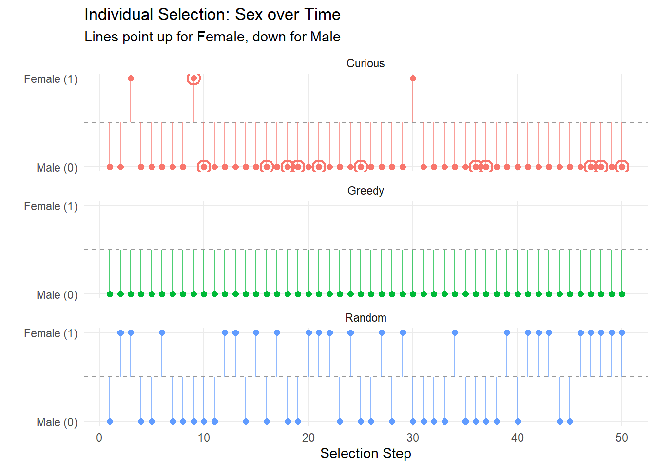
In this we start to see the actual concern with that was highlighted before – on average, males tend to be easier to predict than females, supposing that the results are seeded with predominantly males to begin.8 The curious method fairs slightly better, owing to the random representation here. Now, this is of course not a perfect representation of the curiousity driven approach (and likely not the best implementation of the greedy approach, either)9. However, this highlights the concern that I have with model-based metrics: there is an encoded desire to select those individuals who are easy to predict, rather than those who are diverse/representative. I have a strong suspicion (albeit, with no experience to justify this) that the curiosity-driven optimal control will be highly effective at finding out these ways to exploit, closely tracking with the greedy algorithm in the long-term. If this is the case, then I do think we need to be quite cautious.
Brainstorming on Future Considerations
These simulations, I think, have brought forward two primary points to consider from my perspective. First is the recognition of CDOC as a metaalgorithm in our context; without the added clarity of the underlying purpose, or even the underlying techniques, I am not sure how to assess whether it is working well. Second is the recognition that metrics that are based on performance may incentivise the selection of “easy” rather than “diverse” individuals. I think both points are worthy of further thought.
Fixed or Developing Model
One thing that is worth thinking about is whether we are working from a place with one fixed model (as in the simulations above) or if instead we are trying to determine the best structure for the underlying model. If we imagine that the model being used is completely fixed (such as a linear regression with a given set of predictors), then it is not immediately clear to me how to best have CDOC function for our purposes. In this context, the researchers have already identified what they wish to consider (in terms of demographic diversity) and our goal is to simply fit this model the best that we can. If we had a validation set, we could focus on predictive accuracy on the validation set, but having a validation set feels challenging. Alternatively, we could consider something like power or p-values, though, I think that in the absence of random selection these tools would need to be deeply analyzed for validity.
Alternatively, if we consider the model needing to be discovered, this seems to track better with how I understand the goals, though, it remains complex to think about what the cost function metric is. The rationale here is that, if there is an underlying “model discovery” component, then the need to consider diversity naturally emerges during the recruitment/fitting procedure. The researchers may not think that sex matters (for instance), but if the true model ought to have sex considered, then hopefully this could be discovered. Unfortunately, there is not a one-size-fits-all approach to discovering what model makes the most sense, and as such, this may be difficult to formalize for the setting.
One point to make is that, if we are in a middle-ground of using techniques that do not require explicitl, a priori specification, this may be less of a cocnern. For instance, if we are using a neural network for prediction, this can begin to use all features passed to it, without the explicit need to specify these as important. However, even in such a setting, the concrete measurement to use is not immediately clear to me.
A First Pass at an Alternative
One technique for model selection is using penalized regression. For instance, LASSO regression adds an L1 penalty to the standard cost function in linear regression; this has the consequence of pushing the coefficient on unnecessary variates to \(0\), enforcing a sparsity that is only overcome through sufficient gain in model performance. We might envision a researcher using the fully saturated model (all predictors and their interactions), but fitting with LASSO. This will force most coefficients to zero, leaving only those (or those interactions) that are linearly useful for the outcome of interest. With every new datapoint, the model may change dramatically, deeming previous factors that were important, unimportant, or vice versa.
What if we considered a measure of the diversity of the predictors, in the dataset, that are actually selected by LASSO. Suppose that we define \(\Sigma\) to be the estimated covariance matrix for data, across all variables that have a non-zero estimated coefficient in the LASSO regression. Then, we could consider something like \(\text{det}|\Sigma|\) as a measure of its overall size or volume – larger values would suggest more diversity. Thus, we may look to maximize this quantity. This should be increased by either (1) having more non-zero coefficients [suggesting that new patterns were discovered], or (2) having sufficiently diverse representation among the factors that are already present.
There are some definite concerns with this metric: for instance, it does not consider the scale on which the different predictors are measured, there may be weird noise that arises using a covariance matrix with interactions, and it is not clear to me (though it seems possible) whether there would still be an “extreme bimodal preference” for maximizing the determinant. Still, this would combine both an idea of model fitting alongside an explicit diversity measure, which feels like it is stepping in the right direction.
Some Other Considerations
There is no particular order, but some additional notes here:
- Expected Model Change: This comes from active learning. It is essentially just a difference in the estimated parameters by the model. We could try applying the same thing to the LASSO problem, or similar, where the model is then incentivised to explore the space rapidly.
- Information Theory Concepts: I am always cognizant of not re-encoding curiosity within the algorithm, but in this case something like information gain measures the surprise of the next individual; is this what we are actually after?
- Causal Inference/Precision Medicine: One thing that comes up often in the elevator pitch is an idea of “personalized medicine”. We want to give the right treatment, to the right person, at the right time. Ultimately, if this is what we are looking towards, it may be useful to consider CDOC as a metaalgorithm for some specific model in the realm of precision medicine; this is a big area, but is where I work, and so I know it fairly well. It is important to note that precision medicine is done lots, and there are plenty of different methods to give this. This does not mean that researchers will recruit the right individuals, of course, but if we want to be in this field, then it is perhaps worth expanding on this.
Footnotes
This would lead to (at least) two types of problems, where (1) you want to make sure that your validation set is sufficiently diverse, and (2) it reduces the amount of data you have to actually work with, but if the goal is ultimately out-of-sample prediction, it tends to be a useful starting point.↩︎
I am using https://www.webmd.com/heart-disease/what-is-cardiac-troponin-test as a reference, which suggests that for high-sensitivity troponin I for males, usual levels are \(\leq 20\) nanograms per litre.↩︎
Perhaps not after the first individual, but likely overtime.↩︎
I think that this point has actually unlocked something that is key to me. I will include more details later on, but at this point, I think that the operative question is whether we are trying to optimize the performance of a fixed underlying model (at which point I think we need to turn to validation data) or if we are trying to discover what model would most effectively map on to the real-world.↩︎
It also has the benefit of not being explicitly optimized by the fitting of the logistic regression.↩︎
Note: the code is a little messier here to try to speed up the greedy search. Without it, we would not be able to (in a timely manner) check each point’s MSE.↩︎
There is an interesting pattern after the second random selection where a set of values that are close by the previously selected value are selected in sequence. This seems to suggest that there was learning in this region going on, but afterwards, it feel back.↩︎
Note, I would expect that as the number of individuals continue to progress, the greedy algorithm would eventually outpace the random; it is fairly noisy after \(50\) steps, still.↩︎
For instance, we could consider some level of other consideration, e.g., males with high/low troponin; females with high/low troponin.↩︎