The Bootstrap, Jackknife, and Remeasurement Techniques
Author
Dylan Spicker
Parametric Techniques
Monte Carlo techniques operate through the assumption that we know the underlying distribution that is required, and then we sample from this. Framed in this regard we can call the Monte Carlo techniques that we explored parametric. Parametric methods are the statistical techniques that we perform in which we make assumptions regarding the underlying distributions and work from there. Parametric techniques are widely used: maximum likelihood estimation is a parametric estimation technique; t-tests are parametric hypothesis tests; certain inferential procedures in linear regression are parametric techniques; confidence intervals for the sample mean are parametric. In each of these cases we make an assumption regarding the distribution that our data follow, and then using this distributional assumption, derive theory for the behaviour of the statistical technique. When introducing Monte Carlo simulation we discussed how these techniques could be used to test the performance of parametric techniques when distributional assumptions are invalid.1
Parametric techniques have seen incredible uptake in part due to their efficacy, in part due to their efficiency, and in part because they are easy. There are certain procedures which, while making parametric assumptions, have been used to great effect and as a result continue to see wide use. Parametric procedures, when used correctly, will be more efficient (meaning lower variance, better MSE, functioning with smaller sample sizes, etc.) than techniques which do not make distributional assumptions; in a sense, the distributional assumption allows us to import extra information, which can substitute for having more data. Finally, the ease of development of parametric techniques should not be overlooked. To derive the validity of, for instance, the \(t\) testing procedure can be done without much hassle in an undergraduate mathematical statistics courses, and it is expected that maximum likelihood estimators can be derived by most students finishing a statistics degree. This ease of development is a feature, certainly, and in situations where it is further supported by the first two benefits this can render parametric techniques to be quite useful. But there’s one pressing issue.
In the “real world”, we probably do not know the distribution that data will follow, if they are to follow a nice distribution at all.
Nonparametric Techniques
Enter nonparametric techniques. By contrast to parametric methods, nonparametric methods are those which do not make explicit distributional assumptions in order to guarantee their efficacy. They make restrict attention to features of a distribution, or to classes of distributions, but they do not explicitly say which distribution the data come from. In this sense, by guaranteeing the validity of the nonparametric technique, we need not check the distribution of our data for conformity to some standard, and can instead rely on the generality of the method. To my ears, nonparametric techniques sound like magic. As a first step of demystifying this, it is helpful to acknowledge that there are several nonparametric techniques with which we are already familiar.
Example 1 (Nonparametric Mean Estimation) Suppose that we take \(X_1,\dots,X_n \sim F\), for some distribution \(F\). Suppose that we assume that \(\theta(F) = E[X_i] < \infty\), which is to say that \[\theta(F) = \int_{\mathbb{R}}xdF(x) < \infty,\] then a nonparametric estimator for \(\theta(F)\) is the sample mean. Specifically, \[\frac{1}{n}\sum_{i=1}^n X_i \stackrel{p}{\longrightarrow} \theta,\] for any \(F\) (with finite expectation).
Example 2 (Nonparametric (Linear) Conditional Mean Estimation) Suppose that we have some random quantity, \(X\), which is related to another random quantity \(Y\) via \[Y = \beta_0 + \beta'X + \epsilon,\] where \(\epsilon\perp X\) and \(\epsilon \sim F\). Suppose that \(E[\epsilon] = 0\)2 and that the variance, \(\text{var}(\epsilon) < \infty\), but that otherwise the distribution is unspecified. If we view \(\theta(F) = (\beta_0, \beta)'\), then, the ordinary least squares estimators give a nonparametric estimate for \(\theta(F)\). Specifically, taking \(\widetilde{X}\) to be \(X\) with a column of ones added onto it, \[\widehat{\theta} = (\widetilde{X}'\widetilde{X})^{-1}\widetilde{X}'Y \stackrel{p}{\longrightarrow} \theta(F).\] Thus, linear regression is a valid procedure assuming the correct specification of the model for the conditional mean, without assuming normality of the errors.
The benefits of nonparametric inference are clear and substantial. One major drawback to nonparametric techniques, in general, is the requirement of larger sample sizes. As a general rule, nonparametric techniques require larger sample sizes in order to produce acceptable results than their parametric counterparts. The caveat here is that this is true only when the parametric techniques are correctly specified. Still, this means that if your data are small it will (generally) be the case that finding an appropriate parametric technique will yield more desirable results than using a relevant nonparametric method. With that said, growing sizes of data, improved computational capacity, and the ever present uncertainty of the appropriateness of parametric techniques render nonparametric methods of central importance to modern statistical theory. It would be possible to take an entire course in nonparametric statistical procedures; we will content ourselves with a few subsections.
The Empirical CDF
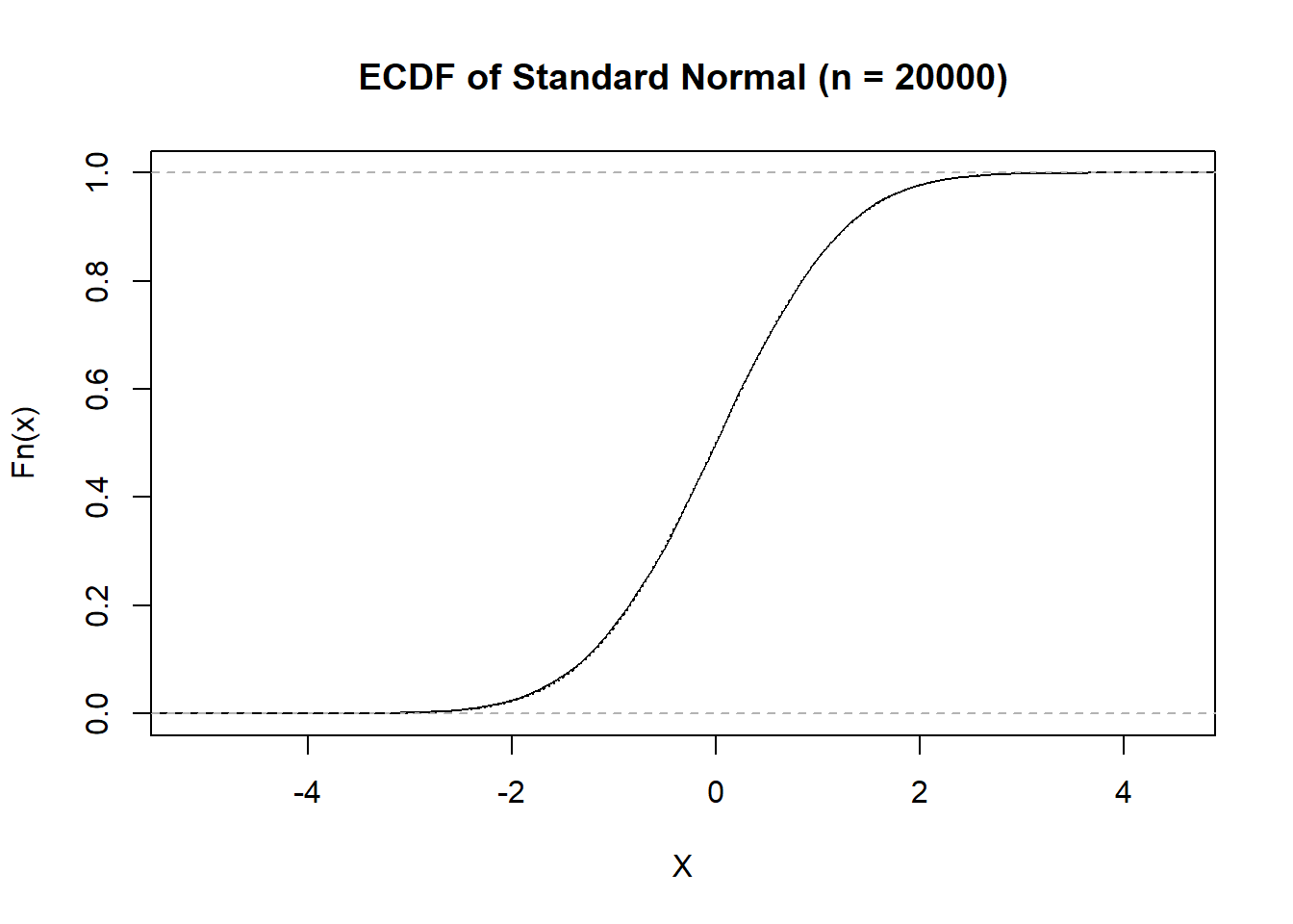
One centrally important idea in nonparametric estimation is that of the empirical CDF. The empirical CDF is a nonparametric method for estimating the CDF of a distribution, given observations from an unknown distribution. The idea is fairly intuitive: we will take the empirical CDF to be the proportion of data points observed below any given threshold. That is, if we observe \(\{x_1, x_2, \dots, x_n\}\) then to estimate \(F(x) = P(X \leq x)\) we count the number of \(x_i \leq x\), and divide by \(n\). The empirical CDF is denoted \(\widehat{F}_n\), where the \(n\) is included to emphasize the dependence on the size of the sample. Mathematically we have \[\widehat{F}_n(x) = \frac{1}{n}\sum_{i=1}^n\mathbb{1}(x_i \leq x),\] where \(\mathbb{1}(\cdot)\) is an indicator function.3
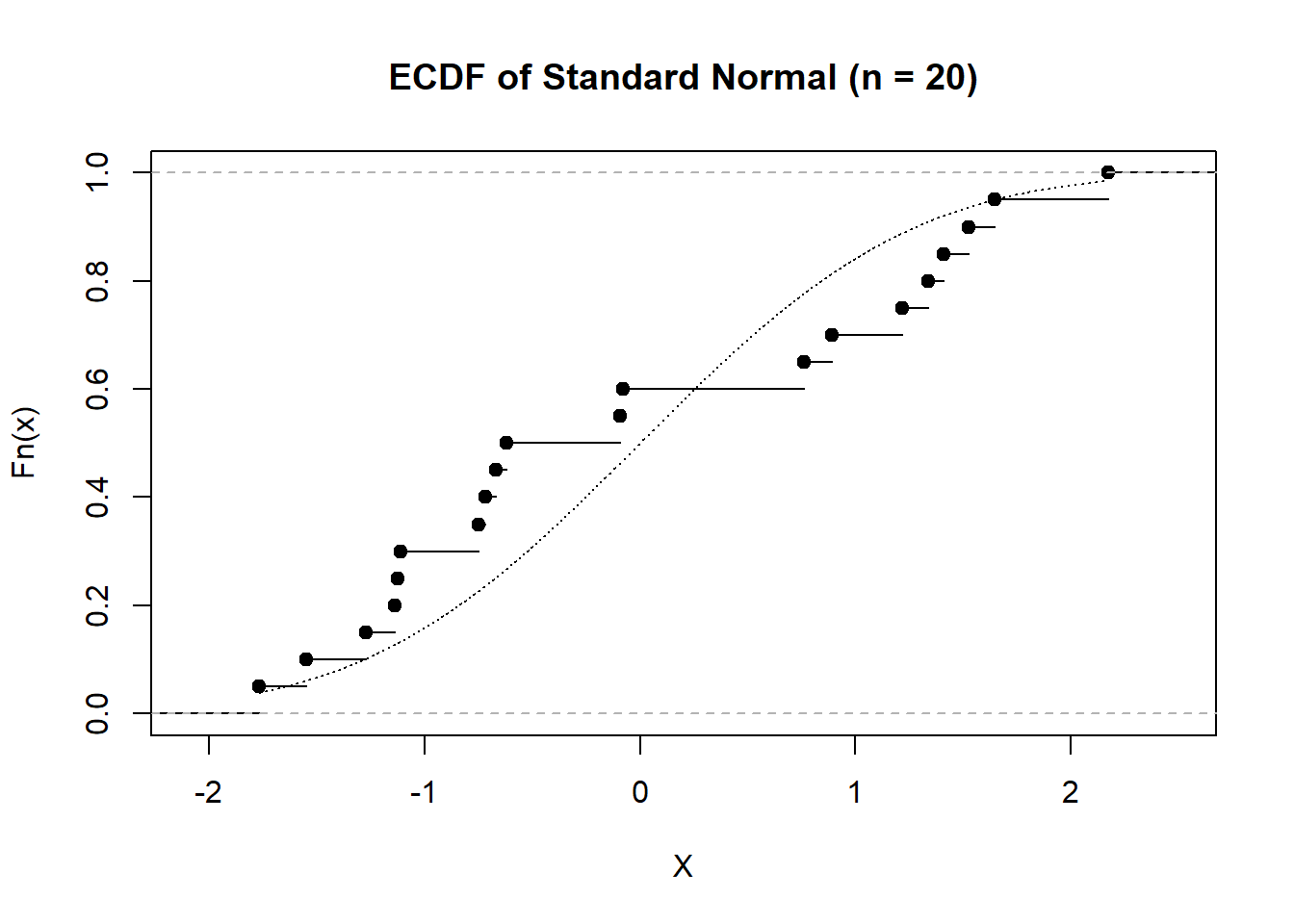
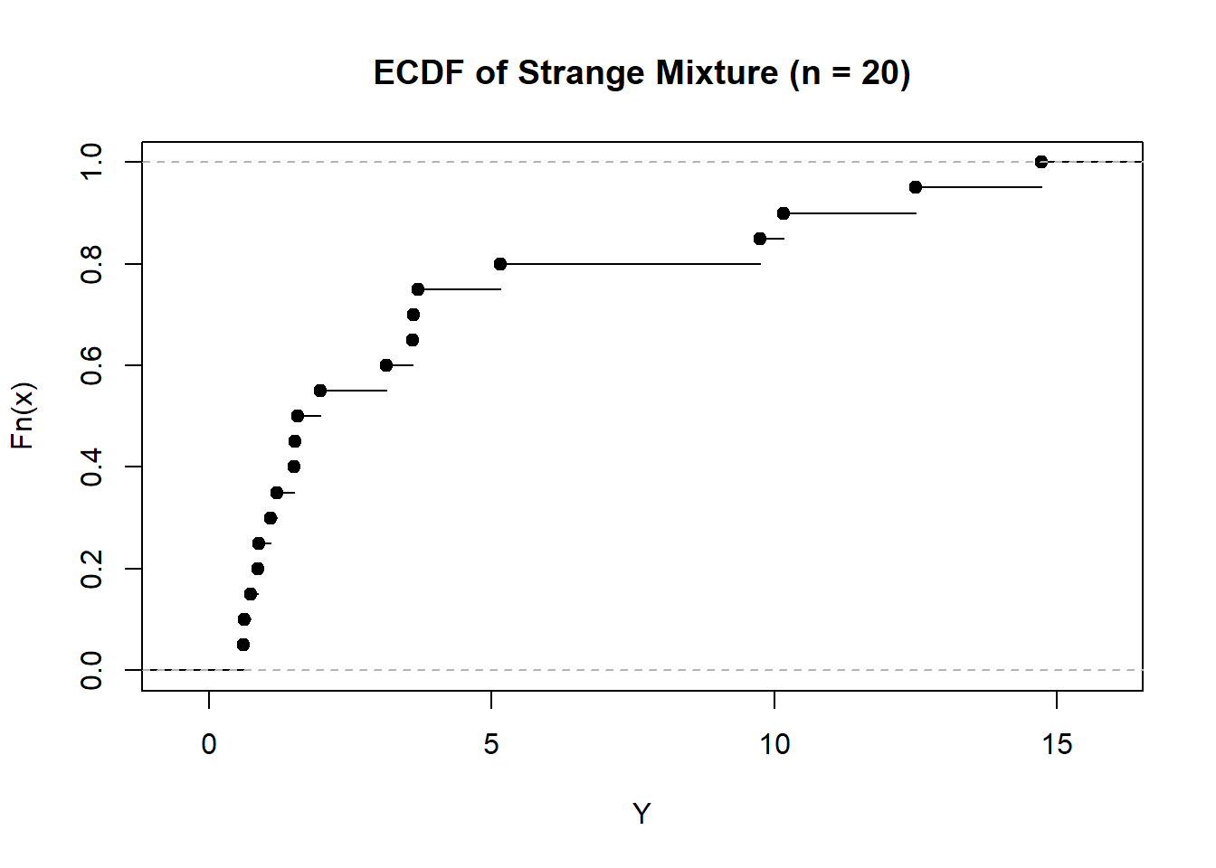
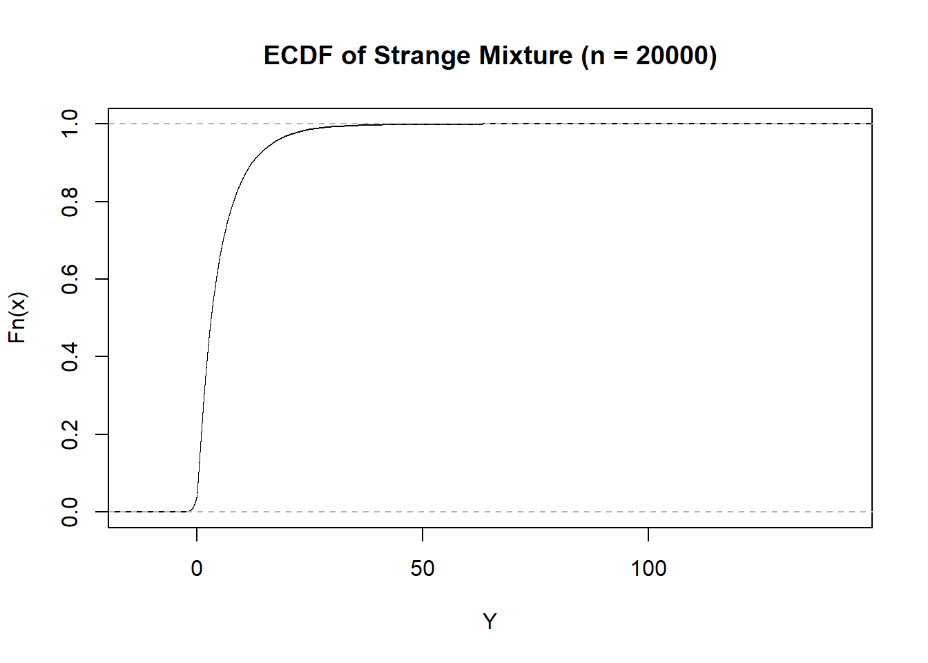
The empirical CDF does not make any distributional assumptions. In fact, it need not make any restrictions whatsoever on the distribution since every random variable has a CDF. In R, given a data set, we can estimate the empirical CDF via the ecdf function.
# Generate some data set.seed(31415) X <-rnorm(20)Y <-rnorm(20)*rbinom(20, 1, 0.5) +rpois(20, 5)*rexp(20)# Compute the ECDFFhatX <-ecdf(X)FhatY <-ecdf(Y)# Plot themplot(FhatX, xlab ="X", main ="ECDF of Standard Normal (n = 20)")# Add the standard normal CDF to thisx <-seq(min(X), max(X), length.out =5000)lines(pnorm(x) ~ x, lty =3)plot(FhatY, xlab ="Y", main ="ECDF of Strange Mixture (n = 20)")
The empirical CDF is, itself, a valid cumulative distribution function. Specifically, if we imagine a discrete distribution which puts probability mass of \(\dfrac{1}{n}\) at each of the values \(\{X_1,X_2,\dots,X_n\}\), then the corresponding distribution will have a CDF given by \(\widehat{F}_n(x)\). As a result, when we talk of the empirical CDF, we can consider either the implied population distribution (\(F\)) which the empirical CDF is an estimator of, or we can talk of the empirical distribution itself. In this sense, we can view the observations, \(X_1,\dots,X_n\), as though they are themselves a finite population from which sampling may occur.
Theoretical Properties of the ECDF
Studying the ECDF in depth is beyond the scope of this lesson, however, there are some theoretical results that are worth acknowledging. First, fix a value \(x\). Notice that for any fixed value of \(x\), the ECDF is simply a sample average of an indicator function. We know that \(0 \leq E[\mathbb{1}(y)] \leq 1\) for any argument \(y\), since the indicator itself is bounded on the interval, and as a result we can apply the laws of large numbers. Specifically, we get that, as \(n\to\infty\), \[\widehat{F}_n(x) \stackrel{a.s.}{\longrightarrow} F(x),\] for all \(x\). This is a claim about pointwise convergence. At every input \(x\), we get the correct value eventually, possibly with its own speed in \(n\).
Still considering the estimation of any given point, we can invoke the Central Limit Theorem, since this is again a sample mean. Notably, \(\mathbb{1}(X \leq x) \sim \text{Bern}(F(x))\). As a result, we have \(E[\mathbb{1}(X \leq x)] = F(x)\) and \(\text{var}(\mathbb{1}(X\leq x)) = F(x)(1-F(x))\). Taken together, with an appeal to the CLT gives \[\sqrt{n}(\widehat{F}_n(x) - F(x)) \stackrel{d}{\longrightarrow} N(0, F(x)(1-F(x))).\] This gives the ability to conduct inference on any particular point estimate, form confidence intervals, and so forth.
While these pointwise results are comparatively easy to see, and are useful in their own right, stronger results exist. In particular, we can appeal to the Glivenko-Cantelli theorem to claim the following uniform converge.
Theorem 1 (Glivenko-Cantelli Theorem) Define the sup-norm to be \[\vert\vert \widehat{F}_n - F\vert\vert_\infty = \sup_{x\in\mathbb{R}}|\widehat{F}_n(x) - F(x)|.\] That is, the sup-norm is the maximum distance between the estimator and the truth, across all possible input values. Then, we can claim that, as \(n\to\infty\), \[\vert\vert \widehat{F}_n - F\vert\vert \stackrel{a.s.}{\longrightarrow} 0,\] giving uniform almost sure convergence to \(0\).
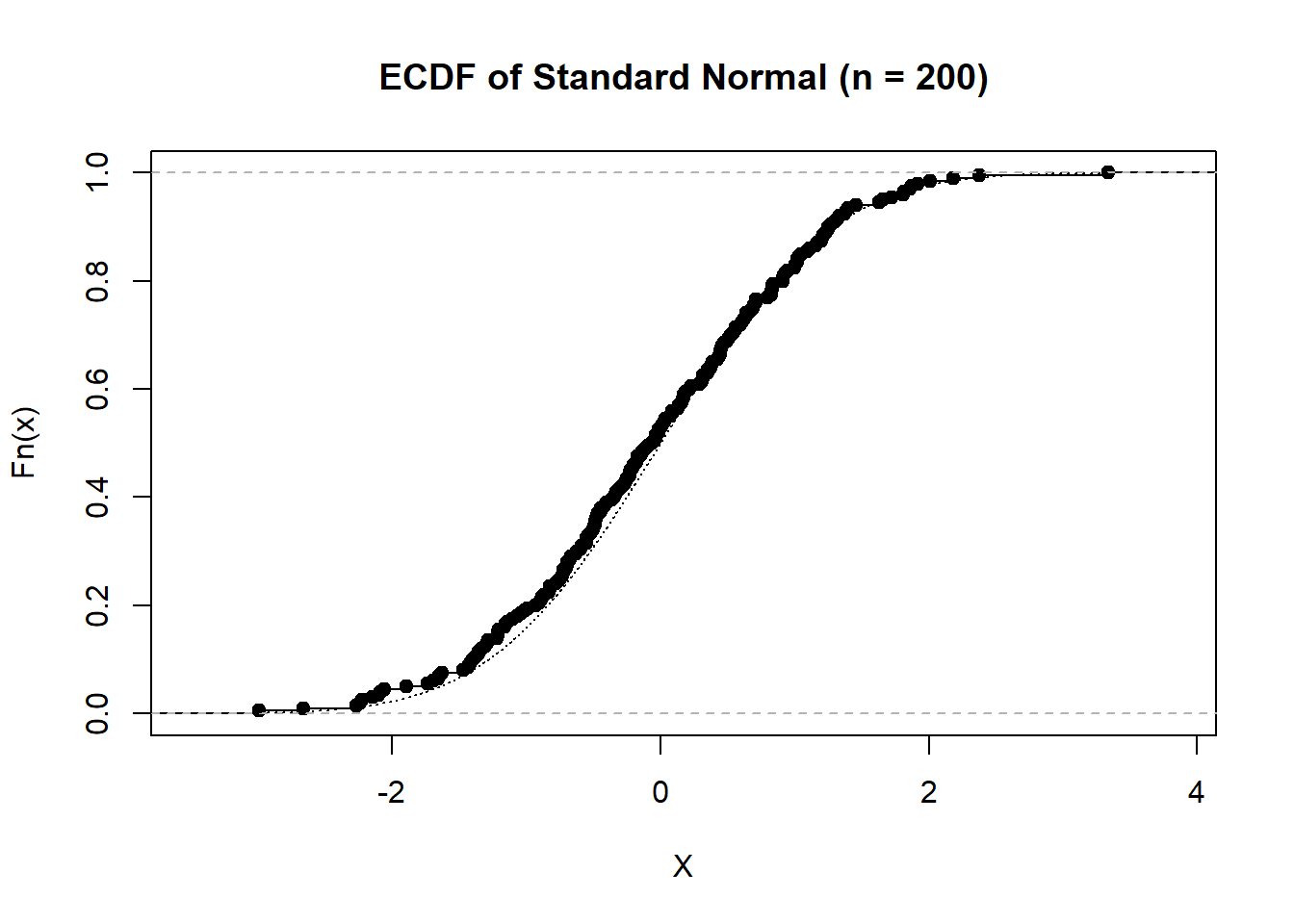
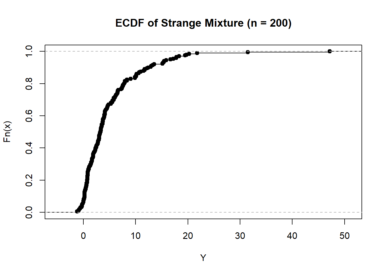
This result is stronger than pointwise convergence.4 The results regarding uniform convergence can be extended to distributional results5 and give rise to the Law of Iterated Logarithm, which specifies the rate of convergence of the ECDF. These results are interesting, and very useful, but beyond our discussion presently. Still, we can take the collection of these results to mean that, as the sample size grow, the ECDF will be a strong estimator for the true CDF, regardless of the underlying distribution.
# Run the same plotting as before, but this time with three different sample sizesns <-c(20, 200, 20000)# Generate some data set.seed(31415) for (n in ns){ X <-rnorm(n) Y <-rnorm(n)*rbinom(n, 1, 0.5) +rpois(n, 5)*rexp(n)# Compute the ECDF FhatX <-ecdf(X) FhatY <-ecdf(Y)# Plot themplot(FhatX, xlab ="X", main =paste0("ECDF of Standard Normal (n = ", n, ")"))# Add the standard normal CDF to this x <-seq(min(X), max(X), length.out =5000)lines(pnorm(x) ~ x, lty =3)plot(FhatY, xlab ="Y", main =paste0("ECDF of Strange Mixture (n = ", n, ")"))}
The Plug-in Principle
While the ECDF is useful in its own regard for estimating distributions, the true utility of it6 stems from the plug-in principle. Roughly speaking, the plug-in principle is a technique for finding estimators for quantities of interest, nonparametrically, in a general technique. The idea to frame the parameter of interest as a functional of the distribution function: that is, we specify \(\theta(F)\) to be a mapping from the CDF of the true data to the real numbers. So, for instance, we can view \[E[X] = \theta(F) = \int_{\mathbb{R}} xdF(x),\] where once you know the CDF you also know the mean. Then, with this framing of the parameter, we take \[\widehat{\theta}_n = \theta(\widehat{F}_n) = \int_{\mathbb{R}} xd\widehat{F}_n(x) = \frac{1}{n}\sum_{i=1}^n X_i.\]
Suppose that we have \(X_1,\dots,X_n \stackrel{iid}{\sim} F\), and we wish to estimate the variance of \(F\). The functional for the variance is given by \[\theta(F) = \int_{\mathbb{R}} (x - E[X])^2dF(x) = \int_{\mathbb{R}} (x - E_F[X])^2dF(x),\] where \(E_F[X]\) emphasizes that the integral is with respect to the distribution, \(F\). Thus, the plug-in estimator for variance has us replacing \(F\) with \(\widehat{F}_n\), giving \[\widehat{\theta} = \theta(\widehat{F}_n) = \int_{\mathbb{R}} (x - E_{\widehat{F}_n}[X])^2d\widehat{F}_n(x) = \frac{1}{n}\sum_{i=1}^n (X_i - \overline{X})^2.\]
This plug-in principle can be quite useful for generating estimators which do not make strong assumptions regarding the underlying distribution. The estimators are not guaranteed to perform well, or to be particularly efficient (in the sense of requiring large sample sizes, for instance), however, it provides a starting point for analysis. The general principle is to compute \(\theta\) for the empirical distribution, and then use the fact that the empirical distribution is estimating the population distribution, in order to claim the estimator as valid for the underlying quantity of interest.
Sampling from the Empirical Distribution (Resampling)
Suppose that we consider the empirical distribution, given some sample \(\{X_1 = x_1, X_2 = x_2, \dots, X_n = x_n\}\). That is, we are fixing in place a discrete probability distribution, and considering that as the distribution of interest. Imagine that we have an parameter of interest, \(\theta(\widehat{F}_n)\). Suppose that we wanted to estimate \(\theta(\widehat{F}_n)\) via a sample of size \(n\) from the empirical distribution. Of course, if we already know all of the \(X_1,\dots,X_n\) we could just compute \(\theta(\widehat{F}_n)\) directly, but if we imagine not knowing precisely the empirical distribution, we may wish to get at this via samples. A sample, \(Y_1,\dots,Y_n\stackrel{iid}{\sim}\widehat{F}_n\) could be used, directly with \(\theta\), to estimate \(\theta(\widehat{F}_n)\). If we could do this repeatedly, we could estimate the variance of the estimator via Monte Carlo techniques. The only thing that remains for this is to form a technique for sampling from the empirical distribution.
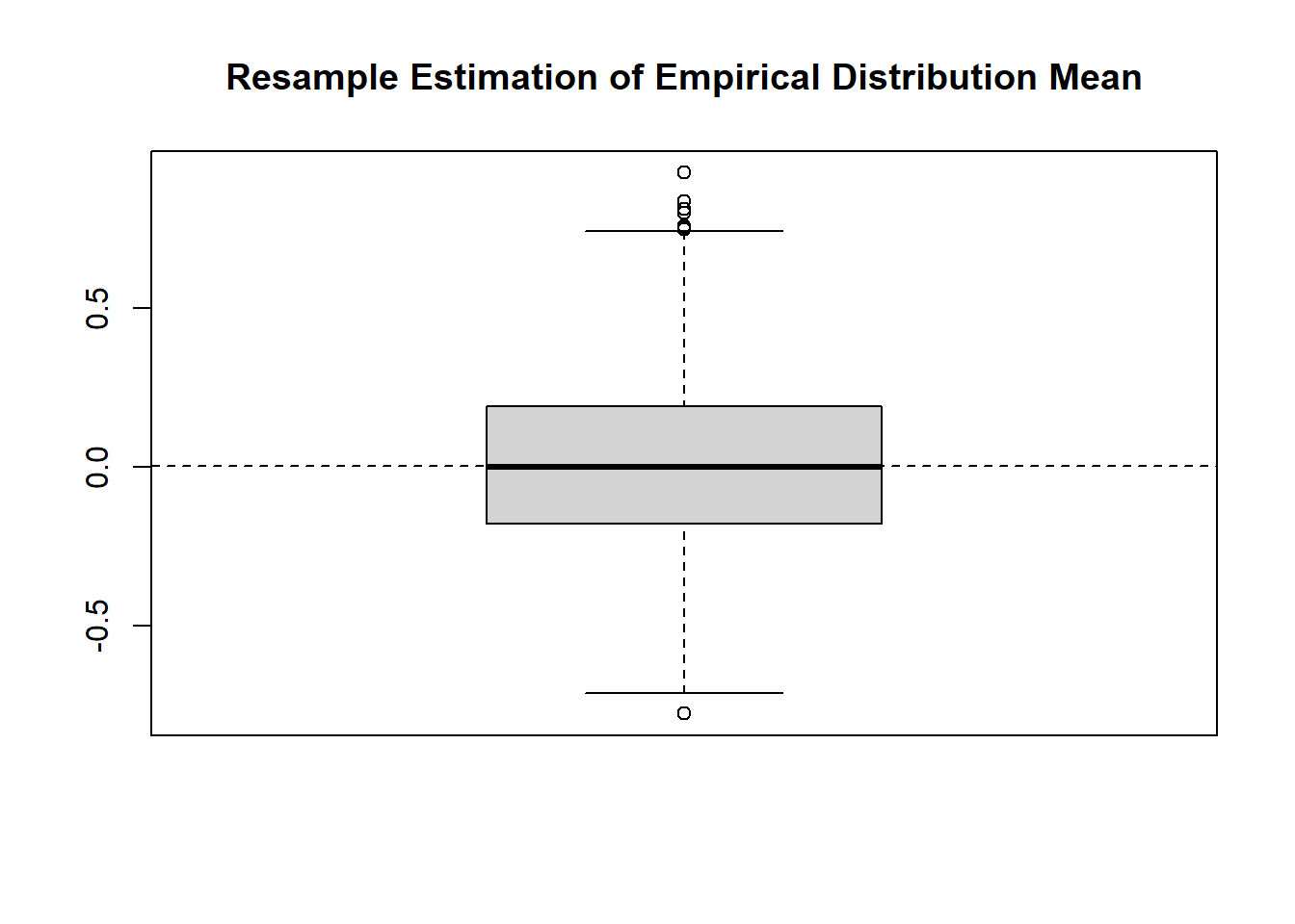
If we have observations for each \(X_i\), then we can sample from this distribution by simply sampling from the list of possible values with replacement. That is, we select each of the observed values with probability \(\dfrac{1}{n}\), independent of all of the other draws that have been made. This process is refered to as resampling as generally it is applied to an existing sample of data. Doing so allows us to work with iid samples from the empirical distribution, forming estimators and estimating their variance.
n <-20resamples <-2000set.seed(31415) ## Generate the original sampleX <-rnorm(n)# Print out the sampleprint(sort(X))## [1] -1.77141948 -1.54854561 -1.27323204 -1.13792539 -1.12539193 -1.11198716## [7] -0.74837846 -0.72021480 -0.66820178 -0.61999643 -0.09450125 -0.07902725## [13] 0.76253633 0.89166252 1.21616823 1.33643937 1.40846809 1.52641110## [19] 1.64701288 2.17590620## Find the True Mean of the Empirical Distributionmu_ed <-mean(X)# Monte Carlo Re-samplingresults <-matrix(nrow = resamples, ncol =1)for (ii in1:resamples) { resample <-sample(X, n, replace =TRUE) results[ii,1] <-mean(resample)}## Show the Boxplot of the Meanboxplot(results, main ="Resample Estimation of Empirical Distribution Mean")abline(h = mu_ed, lty =2)
According to this simulation, the estimated variance of the estimator is 0.0761332. When framed through the empirical distribution, this Monte Carlo approach is fundamentally no different from our previous approaches; the alteration is surface level. Instead of simulating from a parametric distribution, we sample from a discrete distribution described by the values that happened to be viewed. However, it turns out that this procedure of resampling becomes an incredibly powerful statistical technique.
The Nonparametric Bootstrap
Suppose that in order to estimate some parameter, \(\theta(F)\), we use \(\widehat{\theta}\) computed on a sample. Based on the above discussions, we may view \(\widehat{\theta}\) as a parameter of the empirical distribution, \(\widehat{F}_n\). In this light, we can use the aforementioned resampling to understand how estimators of this parameter (of the empirical distribution) would behave. Notably, by forming resampled datasets, \(X_{b1},\dots,X_{bn}\), for \(b=1,\dots,B\) we can understand the variability of these estimators. But remember that the estimator \(\widehat{\theta}\) is an estimator of the population parameter \(\theta(F)\). As a result, the resampled estimates serve as plausible realizations for estimates that could have been seen as estimates of \(\theta(F)\). This process is known as the nonparametric bootstrap, or simply the bootstrap.
To summarize the proposed procedure:
Take a sample from an unknown population distribution, denoted \(X_1,\dots,X_n\) from \(F\).
Calculate an estimate for the parameter of interest, \(\theta(F)\), based on some estimator, \(\widehat{\theta}\).
For \(b=1,\dots,B\):
Form a resampled dataset, \(X_{b1}, X_{b2}, \dots, X_{bn}\).
Calculate \(\widehat{\theta}\) on the resampled datasets, giving \(\widehat{\theta}_b\).
Use the set of \(B\) resampled estimates to understand the variability of the estimator.
Bootstrap Variance Estimation
With the collection of \(B\) estimators, one reasonable step to take is to estimate the variance of \(\widehat{\theta}\) using the sample variance of \(\widehat{\theta}_b\), namely, \[\widehat{\text{var}}(\widehat{\theta}) = \frac{1}{B-1}\sum_{b=1}^B (\widehat{\theta}_b - \overline{\theta}_b)^2,\] where \(\overline{\theta}_b = B^{-1}\sum_{b=1}^B \widehat{\theta}_b\).7 This also gives us the capacity to estimate the standard deviation for the estimator.
The variance of an estimator is often an important component in assessing its performance. Suppose, for instance, that we know that an estimator is unbiased, but where we are unsure of its variability. In that case, the bootstrap estimator of variance can be leveraged to quantify our uncertainty. Note that the bootstrap approximation has errors arising from two different sources: first, there are the Monte Carlo errors associated with the fact that \(B\) is finite, and as a result, there is uncertainty in the resampled estimates. The second source of error stems from the fact that \(n\) is finite, and thus \(\widehat{F}_n\) is an approximation to \(F\). In practice, we can take \(B\) to be as large as is required to really only be concerned regarding the second source of error.
Example 3 (Minimum of Quadratic Function) Suppose that \[Y = \beta_0 - \beta_1x + \beta_2x^2 + \epsilon,\] where \(\epsilon \sim N(0,\sigma^2)\). If \(\beta_0, \beta_1, \beta_2 > 0\), then the minimum occurs at \(x = \dfrac{\beta_1}{2\beta_2}\), and so we may choose to estimate the minimum point via the ratio of the regression coefficients.
To demonstrate the variance estimation we consider two simulations. First, we perform Monte Carlo directly, demonstrating the variability of the estimator based on repeatedly performing the experiment. Then, we use bootstrap to estimate the variance of the estimator.
set.seed(31415) n <-100mc_reps <-2000bs_reps <-10000beta0 <-2beta1 <-3beta2 <-3/2sigma <-1opt <--beta1/(beta2 *2)# Monte Carlo Replicationsmc_results <-matrix(nrow = mc_reps)for (ii in1:mc_reps) {# Generate Data X <-runif(n, -1, 6) Y <- beta0 + beta1*X + beta2*X^2+rnorm(n, 0, sigma)# Fit Model lmfit <-lm(Y ~ X +I(X^2)) mc_results[ii, 1] <-coef(lmfit)['X']/(2*coef(lmfit)['I(X^2)'])}# Bootstrap SamplingX <-runif(n, -1, 6)Y <- beta0 + beta1*X + beta2*X^2+rnorm(n, 0, sigma)bs_results <-matrix(nrow = bs_reps) # Get the Estimateest_lmfit <-lm(Y ~ X +I(X^2))theta_hat <-coef(est_lmfit)['X']/(2*coef(est_lmfit)['I(X^2)'])for(b in1:bs_reps) { bs_idx <-sample(1:n, n, replace =TRUE) bsX <- X[bs_idx] bsY <- Y[bs_idx] bs_lmfit <-lm(bsY ~ bsX +I(bsX^2)) bs_results[b, 1] <-coef(bs_lmfit)['bsX']/(2*coef(bs_lmfit)['I(bsX^2)'])}# Output the Resultsunname(theta_hat) # Estimate Value## [1] 0.888966var(mc_results[,1]) # Monte Carlo variance of estimator## [1] 0.004538835var(bs_results[,1]) # Bootstrap Variance of Estimator## [1] 0.004087853
Example 4 (Covariance in Logistic Regression) Whenever we have a binary outcome, \(Y \in \{0,1\}\), we can use an extension to regression techniques to estimate the probability that \(Y=1\) given a set of predictor variables. The most common method for this is logistic regression, the details of which are beyond this course. However, the main idea for our purpose is that in logistic regression we fit a model for \[\begin{multline*}P(Y=1|X) = \pi(X) = \left(1 + \exp(-\beta_0 - \beta_1X_1 - \cdots - \beta_pX_p)\right)^{-1} \\ \implies \log\left(\frac{\pi(X)}{1-\pi(X)}\right) = \beta_0 + \beta_1X_1 + \cdots + \beta_pX_p.\end{multline*}\]
Logistic regression is thus connected deeply to linear regression, and techniques similar to standard regression analyses are capable of estimating the various slope coefficients for the model. Just like with linear regression, we have theory which allows us to estimate the variance and covariance for the various slope estimators, which is typically applied on the basis of asymptotic justifications. In what follows we consider using bootstrap to estimate the variance-covariance structure in a logistic regression model, and compare it to the theoretically derived estimators.
set.seed(31415) n <-5000bs_reps <-20000beta0 <-2beta1 <-3beta2 <-3/2# Data GenerationX1 <-runif(n, -1, 6)X2 <-rnorm(n) Y <-rbinom(n, 1, 1/(1+exp(-1*(beta0 + beta1*X1 + beta2*X2))))# Fit the Standard Modelmodel_fit <-glm(Y ~ X1 + X2, family=binomial(link="logit"))theoretical_cov <-summary(model_fit)$cov.unscaled# Conduct the bootstrap estimatesbs_results <-matrix(nrow = bs_reps, ncol =length(coef(model_fit)))for(b in1:bs_reps) { sample_idx <-sample(1:n, n, replace =TRUE) bsY <- Y[sample_idx] bsX1 <- X1[sample_idx] bsX2 <- X2[sample_idx]# Fit the logistic regression model for bootstrap bs_model_fit <-glm(bsY ~ bsX1 + bsX2, family =binomial(link="logit")) bs_results[b, ] <-coef(bs_model_fit)}bs_cov <-cov(bs_results)round(theoretical_cov, 3)## (Intercept) X1 X2## (Intercept) 0.010 0.009 0.005## X1 0.009 0.027 0.008## X2 0.005 0.008 0.010round(bs_cov, 3)## [,1] [,2] [,3]## [1,] 0.010 0.009 0.005## [2,] 0.009 0.028 0.008## [3,] 0.005 0.008 0.009
Bootstrap Confidence Intervals
While it may be the case that the covariance of an estimator is itself of interest, often we estimate the variance or covariance structure for the purpose of uncertainty quantification. For this purpose we may turn towards confidence intervals. There are several techniques for constructing confidence intervals using bootstrap estimators, with varying levels of theoretical support. They also vary in their ease-of-use or computational complexity. We will talk about several of these.
Approximate Normal-Based Confidence Intervals
If your estimator is known to be asymptotically normally distributed, and the sample size is large enough to justify the use of asymptotic arguments, then you can use the estimated variance (or standard deviation) and construct a normal-based confidence interval as you would for, e.g., the sample mean. That is, you can take \[\widehat{\theta} \pm Z_{\alpha/2}\widehat{\text{S.E.}}(\widehat{\theta}),\] where the standard error is estimated via bootstrap methods. This has the benefit of being connected to much of the statistical theory that we cover throughout statistical training, allowing us to make good use of these developed tools. Unfortunately, the intervals constructed in this way may be invalid both because the bootstrap variance was inaccurate, or because the normal sampling distribution assumption is invalid.
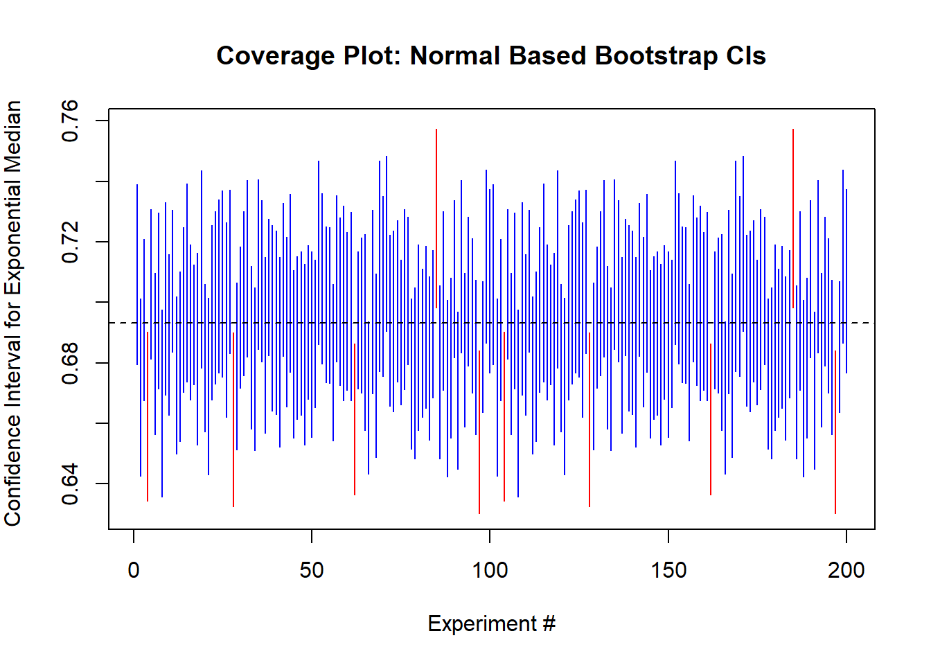
Example 5 (Confidence Intervals for Sample Medians) In what follows we consider confidence intervals formed for the sample median. We draw \(X \sim \text{Exp}(1)\), giving a theoretical median of \(\log(2)\). We will estimate the bootstrap variance, and then form normal confidence intervals around the resulting estimator.
set.seed(31415) n <-5000repeats <-200B <-1000# Bootstrap Resultsresults <-matrix(nrow = repeats, ncol =4)for(ii in1:repeats) { X <-rexp(n) theta.hat <-median(X) bs_results <-matrix(nrow = B, ncol =1)for (b in1:B) { bs_results[b,] <-median(X[sample(1:n, n, replace=TRUE)]) } me <-sqrt(var(bs_results[,1]))*qnorm(0.975) lb <- theta.hat - me ub <- theta.hat + me contain <-as.numeric(log(2) >= lb &log(2) <= ub) results[ii, ] <-c(lb, theta.hat, ub, contain)}
The true median is contained in 0.95 of the intervals. We can see this graphically as follows.
Basic Percentile Based Confidence Intervals
As an alternative to the normal theory confidence intervals, we could use the fact that once we have generated our sequence of bootstrap estimators, \(\widehat{\theta}_1,\dots,\widehat{\theta}_B\), we are in a position where we have already generated a large number of possible realizations for the value of the estimator. If we take this as draws from the true sampling distribution then what we are looking for to form the interval are the percentiles of the sampling distribution. This will allow us to form confidence intervals without reference to the asymptotic normality of the statistic. If we wish to form a \(95\%\) confidence interval, for instance, that we may take the \(97.5\)th percentile for the upper bound, and the \(2.5\)th percentile for the lower bound.
Example 6 (Confidence Intervals for Sample Medians (Percentile Based)) Suppose that we reconsider the previous example with a much smaller sample size \((n=10)\). We can consider the normal confidence intervals in this case.
set.seed(31415) n <-10repeats <-200B <-1000# Bootstrap Resultsresults <-matrix(nrow = repeats, ncol =6)for(ii in1:repeats) { X <-rexp(n) theta.hat <-median(X) bs_results <-matrix(nrow = B, ncol =1)for (b in1:B) { bs_results[b,] <-median(X[sample(1:n, n, replace=TRUE)]) }# Normal Confidence Intervals me <-sqrt(var(bs_results[,1]))*qnorm(0.975) lb <- theta.hat - me ub <- theta.hat + me contain <-as.numeric(log(2) >= lb &log(2) <= ub)# Percentile Based p.ci <-quantile(bs_results[,1], probs =c(0.025, 0.975)) p.contain <-as.numeric(log(2) >= p.ci[1] &log(2) <= p.ci[2]) results[ii, ] <-c(lb, ub, contain, p.ci, p.contain)}
The true median is contained in 0.895 of the intervals via the normal approximation and 0.96 of the percentile-based confidence intervals. As a result, in this setting we get far closer to the nominal coverage by considering the percentile-based confidence intervals, rather than the normal-based ones.
Despite the appealing simplicity of the percentile-based confidence intervals, their justification is largely heuristic. Statistical theory does not typically support the use of this technique, and some authors would go as far as to say that they should never be used. There are several extensions to the percentile technique which, while similar in spirit, are more rigorously justified. As a general rule, these alternative procedures should likely be used.
Better Bootstrap Confidence Intervals
There are several variations on the percentile based bootstrap intervals which may be more theoretically justified or perform better in certain settings. Likely the most prevalent of these is the so-called bias corrected and adjusted for acceleration, or BCa intervals. These are formed in essentially the same manner as the percentile based confidence intervals, however, instead of taking \(\alpha/2\) and \(1-\alpha/2\) for the empirical percentiles, we instead take \(\alpha_1^*\) and \(\alpha_2^*\) given by \[\alpha_1^* = \Phi(\widehat{z}_0 + \frac{\widehat{z}_0 + z_{\alpha/2}}{1 - \widehat{a}(\widehat{z}_0 + z_{\alpha/2})})\quad\text{and}\quad \alpha_2^* = \Phi(\widehat{z}_0 + \frac{\widehat{z}_0 + z_{1-\alpha/2}}{1 - \widehat{a}(\widehat{z}_0 + z_{1-\alpha/2})}).\] Here, \(z_{\alpha} = \Phi^{-1}(\alpha)\), \(\widehat{z}_0\) is a bias correction factor, and \(\widehat{a}\) is an acceleration correction factor.
First, we have that \[\widehat{z}_0 = \Phi^{-1}\left(\frac{1}{B}\sum_{b=1}^B\mathbb{1}(\widehat{\theta}_b \leq \widehat{\theta})\right).\] That is, it is the normal critical value for the percentile at which the estimated value for \(\theta\) falls in the bootstrap distribution. If \(\widehat{\theta}\) is the median of the bootstrap replicates then \(\widehat{z}_0 = \Phi^{-1}(0.5) = 0\). To estimate \(\widehat{a}\), we require a diversion about jackknife estimation.
The jackknife is a technique which existed prior to the bootstrap. In it we are attempting to once again use our sample to estimate the variability of estimators, but instead of resampling, we consider the \(n\) samples of size \(n-1\) which can be formed by leaving out any observation. That is, if for some \(i\), we leave \(i\) out of the sample, we can form \(\widehat{\theta}_{(i)}\) as our estimator computed on the dataset without point \(i\). While this has historically been an important strategy in statistical analyses, and while there are still use cases for the jackknife in a modern analytical toolkit8 Details for how jackknife procedures can be used to estimate the variance or bias associated with an estimator are available in the course textbook (and in similar references).
For our purpose the jackknife technique is relevant as it provides a means for estimating the acceleration parameter, \(\widehat{a}\). Specifically, taking \(\overline{\theta}_{(\cdot)}\) to be the mean of the jackknife estimates, we take \[\widehat{a} = \frac{\sum_{i=1}^n(\overline{\theta}_{(\cdot)} - \widehat{\theta}_{(i)})^3}{6\left[\sum_{i=1}^n(\overline{\theta}_{(\cdot)} - \widehat{\theta}_{(i)})^2\right]^{3/2}}.\] In this case, \(\widehat{a}\) is essentially a measure of the skewness.
Example 7 (Estimating a Ratio of Moments) Suppose that we have \(X \sim F\) from an unknown distribution, and we want to estimate \(\dfrac{E[X]}{\text{var}(X)}\). We can use the simple ratio of sample moments to do so, and then consider various bootstrap confidence intervals for the resulting data.
set.seed(31415) n <-500repeats <-200B <-1000# Bootstrap Resultsresults <-matrix(nrow = repeats, ncol =3)for(ii in1:repeats) {# Generate Data X <-rgamma(n, shape =2, scale =3) truth <-1/3 theta.hat <-mean(X)/var(X)# Bootstrap Runs bs.results <-vector(mode ="numeric", length = B)for(b in1:B) { bsX <- X[sample(1:n, n, TRUE)] bs.results[b] <-mean(bsX)/var(bsX) }# Jackknife replicates jackknife.results <-vector(mode ="numeric", length = n)for(jj in1:n){ jackknife.results[jj] <-mean(X[-jj])/var(X[-jj]) }# Parameter Calculation z0 <-qnorm(mean(bs.results <= theta.hat)) a.dev <-mean(jackknife.results) - jackknife.results a <- (sum(a.dev^3))/(6*sum(a.dev^2))^(3/2) zs <-qnorm(c(0.025, 0.975)) alpha1 <-pnorm(z0 + (z0 + zs[1])/(1- a*(z0 + zs[1]))) alpha2 <-pnorm(z0 + (z0 + zs[2])/(1- a*(z0 + zs[2])))# Normal Distribution CIs n.ci <- theta.hat +qnorm(c(0.025, 0.975))*sqrt(var(bs.results))# Percentile Based CIs p.ci <-quantile(bs.results, probs =c(0.025, 0.975))# BCa Based CIs bca.ci <-quantile(bs.results, probs =c(alpha1, alpha2))# Save off the CI results results[ii,] <-c( n.ci[1] <= truth & truth <= n.ci[2], p.ci[1] <= truth & truth <= p.ci[2], bca.ci[1] <= truth & truth <= bca.ci[2])}
The resulting empirical coverage for the normal, percentile, and BCa intervals were (respectively) 0.955, 0.935, 0.945. In this context, each appear to do a roughly equivalent job of capturing the uncertainty.
The BCa have at least two major theoretical advantages: first, they are transformation respecting, and second, they are second-order accurate. By transformation respecting we mean that if \((a, b)\) is a confidence interval for \(\theta\), then \((t(a), t(b))\) will be a valid confidence interval for \(t(\theta)\). By second order accurate we mean that the error goes to zero at a rate of \(\dfrac{1}{n}\). By contrast to the other techniques, the percentile methods are transformation respecting but not second order accurate (errors go to zero at a rate of \(\dfrac{1}{\sqrt{n}}\)), and the normal-based confidence intervals are neither.
Bootstrap Bias Estimation
While bootstrap is most commonly used to provide estimates of the variance of estimators, or to form confidence intervals for them, it is also possible to apply the same resampling techniques to estimate the bias of an estimator. Suppose that \(\widehat{\theta}\) is an estimator of interest, for some parameter \(\theta(F)\). The bias of our estimator is given by \[\text{Bias}(\widehat{\theta}) = E_F[\widehat{\theta}] - \theta(F),\] where the expectation is respect to the true population distribution (included for emphasis). In order to estimate this, one may think to use the plug-in principle, giving \[\widehat{\text{Bias}}(\widehat{\theta}) = E_{\widehat{F}_n}[\widehat{\theta}] - \theta(\widehat{F}_n).\]
The second component, \(\theta(\widehat{F}_n)\) is the standard nonparametric estimator for \(\theta\). In order to estimate \(E_{\widehat{F}_n}\), we can use bootstrap resampling. Recall that a bootstrap sample is a draw from \(\widehat{F}_n\). As a result, if we compute \(B\) iid estimates from resamples, then as \(B\to\infty\), \[\frac{1}{B}\sum_{b=1}^B \widehat{\theta}_{b} \stackrel{p}{\longrightarrow} E_{\widehat{F}_n}[\widehat{\theta}].\] Thus, in order to estimate the bias, we can take the mean of our bootstrap replicates and subtract from that the plugin estimator for the parameter of interest.
Example 8 (Estimated Bias of Variance Estimators) The typical sample variance estimator is given by \[\dfrac{1}{n-1}\sum_{i=1}^n(X_i - \overline{X})^2,\] which is selected since it is theoretically unbiased. A slightly more natural estimator is to take \[\dfrac{1}{n}\sum_{i=1}^n(X_i - \overline{X})^2,\] as it takes the form of the sample mean. This estimator, however, will generally be biased. It turns out that taking \[\dfrac{1}{n+1}\sum_{i=1}^n (X_i - \overline{X})^2,\] will typically produce an estimator with even smaller MSE, however, it will have a larger bias. We can use bootstrap to estimate the bias of each of these techniques. Note in this case, \(\theta(\widehat{F}_n)\) is given by \[\dfrac{1}{n}\sum_{i=1}^n(X_i - \overline{X})^2.\]
set.seed(31415)n <-40B <-10000# Generate the DataX <-rnorm(n, 0, 5)# Calculate the estimatorsssd <-sum((X -mean(X))^2)theta.nm1 <- ssd/(n -1)theta.n <- ssd/ntheta.np1 <- ssd/(n +1)# Bias Estimation via Bootstrap## First: bootstrap estimates for each of the estimatorsbs_results <-matrix(nrow = B, ncol =3)for(b in1:B) { idx <-sample(1:n, n, TRUE) bs_ssd <-sum((X[idx] -mean(X[idx]))^2) bs_results[b,] <-c(bs_ssd/(n-1), bs_ssd/n, bs_ssd/(n+1))}# Take the Meanbias.nm1 <-colMeans(bs_results)[1] - theta.nbias.n <-colMeans(bs_results)[2] - theta.nbias.np1 <-colMeans(bs_results)[3] - theta.n
Define the estimators by the constant they are divided by. The theoretical bias for \(n-1\) is \(0\) and the bootstrap estimated bias is -0.0794. The theoretical bias for \(n\) is -0.625 and the bootstrap estimated bias is -0.7743. The theoretical bias for \(n+1\) is -1.2195 and the bootstrap estimated bias is -1.4352. The estimators are not perfect, but they provide a good approximation to the scale of the bias in this setting.
Bootstrap Estimation in R
If you are using R, bootstrap methods are implemented in the package boot. This implements all of the ideas we have discussed, as well as plenty of extensions which are relevant in certain settings.
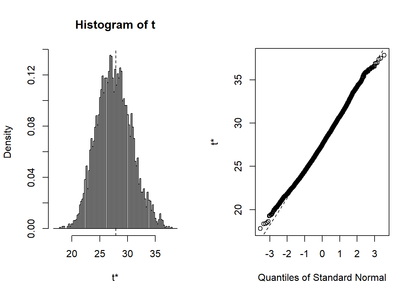
library(boot)# Define statistic to bootstrapfn <-function(X, idx) { sum((X[idx] -mean(X[idx]))^2)/(length(idx) +1) }# Generate Dataset.seed(31415)X <-rnorm(100, 0, 5)# Run the Bootstrapbs_results <-boot(data = X,statistic = fn,R =5000# Number of Replicates )print(bs_results)
The function takes in the data (as a data frame or vector), the statistic (a function which takes in your data as the first argument and a set of indices for the selection as the second), and then umber of replicates. Other optional parameters are given as well. This will return a bootstrap object which contains some information (estimated value of the statistic, standard error, and estimated bias). Note, the bias is only a valid estimate for the bias if your statistic is a plug-in estimator to begin. This object can then be passed to various other functions, such as plot or boot.ci.
BOOTSTRAP CONFIDENCE INTERVAL CALCULATIONS
Based on 5000 bootstrap replicates

CALL :
boot.ci(boot.out = bs_results, conf = c(0.9, 0.95, 0.99), type = c("norm",
    "basic", "perc", "bca"))

Intervals :
Level      Normal              Basic
90%   (23.07, 33.31 )   (22.79, 33.11 )
95%   (22.09, 34.29 )   (21.70, 33.87 )
99%   (20.17, 36.20 )   (19.82, 35.48 )

Level     Percentile            BCa
90%   (22.67, 32.99 )   (23.50, 34.11 )
95%   (21.92, 34.08 )   (22.69, 35.28 )
99%   (20.31, 35.96 )   (21.48, 36.80 )
Calculations and Intervals on Original Scale
Some BCa intervals may be unstable
This makes it easy to calculate any of the different types of bootstrap confidence intervals, at any level of confidence. A major benefit to using the boot package in practice is that it is computationally efficient and can easily be made to be parallelized, in the event of large operations.
Footnotes
We saw, for instance, an example of using the normal distribution to form confidence intervals in place of the \(t\) distribution.↩︎
This is not really an assumption, more of a convenience of notation. If \(E[\epsilon] \neq 0\), then we can take \(\epsilon^* = \epsilon - E[\epsilon]\), and \(\beta_0^* = \beta_0 + E[\epsilon]\) and set up the problem likewise.↩︎
This takes a value of \(1\) if the argument is true, and \(0\) otherwise.↩︎
Consider, for instance, the function \(f_n(x) = \dfrac{x^2}{n}\). We can claim that, for any fixed value of \(x\), \(f_n(x) \to 0\) as \(n\to\infty\). However, consider instead taking \(\lim_{n\to\infty} \sup_x |f_n(x)|\). This will give an indeterminate form. As \(x\) grows we need larger and larger \(n\) to render the sequence convergent.↩︎
Though, this necessitates a discussion of empirical processes, a topic which even I do not have the time to take a diversion for.↩︎
In actual fact, instead of dividing by \(B-1\) for the variance, we will likely just divide by \(B\), but as \(B\to\infty\) there is no material difference.↩︎
For instance, the jackknife is closely related to a technique known as cross validation, and specifically, leave one out cross validation (LOOCV). Cross validation, generally, is a technique for model selection that proceeds by repeatedly fitting models on subsets of the data, and then testing these models on the withheld data.↩︎